A Brief History of Large Language Models
Large Language Models (LLMs) have dominated discussions in machine learning for the past few years, and have transformed the landscape of AI for years to come. This article serves as the prelude to the series “LLMs from Scratch” — a complete guide to understanding and building LLMs. Assuming little background knowledge, the aim is to build an intuitive understanding of how these models work from the ground up, using diagrams, animations, Python code, and the underlying mathematics. APIs and online user interfaces make interacting with LLMs as easy as entering a prompt, but truly understanding the inner workings of these complex models requires a much closer inspection. To set the scene for the articles to come, we will first cover the context behind LLMs: the models that preceded them, their limitations, and how we got to where we are today. In doing so, the goal is to lay out a roadmap for where the series will go. Namely, these articles will cover: every major component of the transformer architecture (the backbone of LLMs), state-of-the-art (SOTA) models such as GPT-4 and Llama 2, how to perform common Natural Language Processing (NLP) tasks with LLMs such as Named Entity Recognition (NER) and topic modelling, and other key topics such fine-tuning and Retrieval Augmented Generation (RAG).
Prelude to the “LLMs from Scratch” series — a complete guide to understanding and building Large Language Models. If you are interested in learning more about how these models work I encourage you to read:
- Prelude: A Brief History of Large Language Models (Current article)
- Part 1: Tokenization — A Complete Guide
- Part 2: Word Embeddings with word2vec from Scratch in Python
- Part 3: Self-Attention Explained with Code
- Part 4: A Complete Guide to BERT with Code
1. Introduction to Transformers
1.1 What are Transformers?
When reading about LLMs, it is impossible to avoid the term “transformer”. It seems as if the two concepts are inseparably linked, and as of now at least, they are. Transformers are type of deep neural network architecture which form the backbone of LLMs today. The architecture was originally introduced in the 2017 paper “Attention is All You Need” — a collaborative effort between Google Brain, Google Research, and the University of Toronto [2]. The goal of which was to improve upon the Recurrent Neural Network (RNN) based models that were popular at the time, particularly for the task of machine translation. That is, translating a sequence of text from a source language (e.g. English) into a target language (e.g. French). The resulting model produced SOTA results, without the restrictions of recurrence-based networks. Transformers are not only restricted to the task of translation, but have also produced SOTA results on a number of NLP tasks such as sentiment analysis, topic modelling, conversational chatbots, and so on. As such, these types of models and their derivatives have become the dominant approach in contemporary NLP. With the release of ChatGPT in November 2022, transformers are perhaps most famous for their use in LLMs such as GPT-4, BERT, and Llama 2.
Since around 2020, transformers have been adapted for use outside the NLP domain. Computer vision models such as Vision Transformer (ViT) perform image segmentation in autonomous driving applications [3], and models such as iTransformer have been used for time-series forecasting [4]. This article will focus on the use of transformers in LLMs.
Note: The term “machine” in “machine translation” is a hold-over from AI terminology in the 1950s/1960s, as it was typical at the time to include “machine” in the title of problems solved by computers. The first widely researched use case of machine translation came about during the cold war, when American computer scientists attempted to build rule-based models to translate Russian texts into English. These early language models worked with limited success and the project was ultimately cancelled, nevertheless the groundwork was laid for future translation efforts. If you are interested in reading more about the history of machine translation, 2M Languages have a great summary on their blog [5].
1.2 Statistical Machine Translation (SMT)
To understand the architectural decisions in the original transformer paper, we first need to understand the problem that the authors were trying to solve. With that in mind, let’s briefly take a look at the history of machine translation, the models developed along the way, and the issues with them that the transformer was designed to solve.
The machine learning landscape was very different before the development of transformers, especially in the field of NLP. After the decline of rule-based systems for machine translation in the 1960s, research stagnated for around 30 years. In the mid 1990s, research efforts were revived and moved towards a statistics-based approach called statistical machine translation (SMT). In this approach, text from the source language is ingested and translated into the target language using an alignment model. This “alignment” refers the process of mapping words or phrases from one language into another, accounting for the order and possible omission/addition of words in the target language. Let’s look at each of these in turn using an example of Japanese to English:
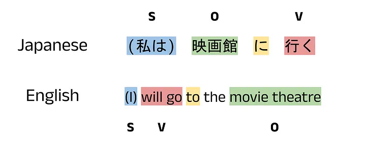
Japanese to English example sentence translation. All images by author unless otherwise stated.
- Word/Phrase Order: Japanese is a subject-object-verb (SOV) language and so verbs are placed at the end of a sentence. English is a subject-verb-object (SVO) language, and so verbs are placed before the object. This means that translating a Japanese sentence word by word into English will give very poor results that are almost always grammatically incorrect. In the example above, the Japanese verb 行く (“to go”) comes at the end of the sentence, but the English translation places the verb before the object “movie theatre”. In this case, the alignment model will need to be trained to correctly order the words according to their function in the sentence.
- Word/Phrase Omission: Japanese often uses context to imply the subject of a sentence. For example, if you are having a conversation with someone about your plans for the day, you don’t need to say “I will go the movie theatre” or “I will go swimming”. It is clear from context that you are the subject of the sentence and so the word for “I” (私) is often dropped. This means that when translating from English to Japanese, it would be more natural to omit “I” in the translation, giving: “will go to the movie theatre” and “will go swimming”.
- Word/Phrase Addition: By the same token, if the model is translating in the other direction from Japanese to English, it would be very unnatural not to include a subject. The model must be able to infer the subject and automatically add in the correct topic for the sentence, thereby adding an additional word that was not in the source sentence. In this case, inserting the subject “I” at the start of each sentence.
There are other times that word omission/addition can occur. For instance, in some languages a concept can be represented by a single word, whereas other languages may require multiple (e.g 映画館 vs “movie theatre”). Another case is the use of indefinite and definite articles such as “a” and “the” in English which do not exist in many east Asian languages. To capture these complexities, aligned-based SMT models made use of many separately designed components. These included a language model to ingest the input sentence, a translation model for producing an output sequence, a reordering model to account for the different word orders of the input and target language, an inflection model to capture the form of the verbs/adjectives used, and so on [6]. Using a combination of many components like this came with challenges. Firstly, a large amount of feature engineering was required (i.e. the input text needed to be pre-processed before being passed to the model). Secondly, frequent human intervention was required to maintain the models, and ensure they worked harmoniously as one unit. Thirdly (and perhaps most importantly), the components needed to be reworked for each language pair, meaning the final model was not a universal translator. For early translation packages, one model would be needed for English to French, another for English to German, and so on. The performance of these statistical language models was mixed, but overall they were successful enough for Google to launch Google Translate in April 2006.
1.3 Early Neural Machine Translation (NMT)
In the early 2010s, advancements in neural networks began to accelerate. Hardware power increased, and so training large neural networks became more feasible. In 2013, Kalchbrenner and Blunsom successfully applied a Convolutional Neural Network (CNN) to translate English into French [7]. Previously CNNs had almost exclusively been used for computer vision tasks such as image recognition and object detection, so this marked a significant change for NLP research. In 2014, researchers across the world independently exploited RNNs for translation as well, producing models with much simpler architectures and SOTA results [8–9]. Overall, these events formed the beginning of what we now call Neural Machine Translation (NMT) — the dominant translation approach today.
1.4 Encoder-Decoder Architecture
The problem of machine translation fits more broadly under the category of sequence-to-sequence modelling, also known as sequence transduction or seq2seq. Sequence-to-sequence models take in a sequence as their input (e.g. a sequence of words forming a sentence, a sequence of pixels forming an image, etc) and output another sequence (e.g. a translation, a caption for an image, etc). In the landmark paper Learning Phrase Representations using RNN Encoder-Decoder for Statistical Machine Translation, the authors demonstrated how a model with two RNNs could capture “both semantic and syntactic structures of the phrases” in the source and target languages for translation [8]. The main idea was that one network could be trained to encode the source text by converting it into embedding vectors, and the other network could be trained to decode the output of the model from embeddings to the target language. These networks were called the encoder and decoder respectively. The idea of separating a model into an encoder and a decoder had been proposed since at least 1997 [10], however training RNNs for such roles was a ground-breaking development.
1.5 Limitations with Early NMT Models
Traditional RNNs suffered from some significant limitations, and so the Long Short-Term Memory (LSTM) model was created to rectify some of these issues [11]. However, LSTMs still use recurrence and so the fundamental issues were not entirely overcome. To produce more robust models, a new architecture was required altogether: hence the development of the transformer. At its core, the transformer was designed to fix the issues with traditional RNN and LSTM-based models. To understand what these problems were and why they came about, let’s briefly look at how RNNs and LSTMs work.
1.6 Recurrent Neural Networks (RNNs):
RNNs are a class of neural networks based on the typical feedforward architecture you may be familiar with. The key difference is that the output of a recurrent neuron is passed back in as an additional input alongside the next value in the input sequence at each time step. For this reason, the flow of information in RNNs is said to be bi-directional, flowing forwards and backwards throughout the network. This distinction is also where the term “feedforward” comes from, to make clear when a network does not use this recurrence.
The animation below shows a recurrent neuron, with a sequence of inputs X. This sequence is made up of values x_t, where t represents the current time step. In an NLP context, the input sequence may be a sentence, where each value is a word embedding. At the first time step, t=0, the input to the neuron is x_0. This input is first processed as usual for a feedforward neuron: the input is multiplied by a weight, w_x, and a bias term, b, is added to form a weighted output. The weighted output is then passed through an activation function, which for recurrent neurons is typically the sigmoid or hyperbolic tangent function, tanh. The output value, y_0, is then passed back into the neuron at the next time step alongside the next value in the input sequence, x_1. This continues for each value in the sequence until all values have been passed into the neuron.
Note: The diagram below shows a simplified case where each word embedding, x_t, is a single number value and not a vector. Therefore, at each time step we can pass in the embedding value and then iterate to the next embedding value using this single neuron. In real models, multiple recurrent neurons are used, with one neuron for each embedding dimensions. These form the input layer for the RNN, and allow vector embeddings to be used to encode each word.
Animation of a recurrent neuron.
y_0 encodes some information about the first value in the sequence, and so is called a hidden state. As t increases, the hidden state encodes more information about the previous values in the input sequence. For our translation task, the network will be passed a sentence one word at a time, and each neuron output will be calculated based on the current word, x_t, as well as all of the previous words in the sentence, encoded in the hidden state, y_t. As always, the weights and bias terms are iteratively improved using backpropagation during training. Layers of recurrent neurons are connected to form the RNN.
1.7 The Problem with RNNs:
RNNs suffer from two main drawbacks:
Exploding and Vanishing Gradients:
- This problem can be understood by recalling the structure of the RNN. Each output of a neuron, yt, is dependent on the previous output of the neuron y{t-1}. If the current output is large (i.e. greater than 2), the next output will be larger. This has a compounding effect over even just a few inputs. Consider a neuron which accepts a sentence of 10 words. A large value of y_0 will generate a larger value of y_1, which compounded over 10 iterations will produce an exponentially large result. This is called the exploding gradient problem. This is not ideal for training a network, as it can cause large, divergent steps in the gradient descent algorithm, rather than small steps converging to optimum weight and bias values. In simple terms, the network will not train well, and so performs poorly. On the other hand, if the current neuron output is small (i.e. less than 1), all subsequent outputs will be smaller, causing the vanishing gradient problem. In this case, the steps made in gradient descent will be too small, and so the weight and bias terms will never converge to optimum values. Again, this will result in poor network behaviour.
Limited Context Window:
- The second problem relates to the hidden state values. For a short sentence, you can imagine that the single floating point value of the hidden state can capture a decent amount of information about the previous words. However for large paragraphs (or entire books), the hidden state values will become less dependent on values from earlier time steps, and capture only the most recent inputs. This is called a limited context window, and in the context of NLP can be thought of as the network “forgetting” earlier words and sentences.
1.8 LSTM Improvements and Drawbacks
LSTMs were designed to address the two issues with traditional RNNs described above, but fundamentally are still a type of recurrent network and therefore suffer from the inherent limitations of such models. In LSTMs, the neurons are often called units to signify the increased complexity of each cell. A cell is made up of three key components: the input gate, output gate, and forget gate. This article won’t delve too deeply into the intricacies of LSTMs, but for purpose of understanding transformers, the key takeaways are that LSTMs improved the size of the context window compared to traditional RNNs. This means that words that occur earlier in the input text are captured more successfully. However, the size of the context window is still limited, so models do not perform well with long input sequences. Additionally, since LSTMs introduce many more parameters that must be learned, training takes much longer when compared to traditional RNNs.
2 Moving Towards Large Language Models
2.1 How Transformers Overcame the Limitations of RNNs and LSTMs
Transformers overcame both of the main issues with LSTMs by using clever architectural design, and exploiting parallel computing. To improve the training time, all values in the input sequence are ingested simultaneously, rather than in series. By processing each word in a sentence at the same time, the model can take advantage of parallel computing and distribute the training workload across many cores of a GPU (or even multiple GPUs). The second major development was the use of the attention mechanism, which is how the model determines which words give context to other words. The use of attention means that the model does not rely on hidden state values that decay over time, but on matrices of attention scores that can be computed directly. Given a powerful enough computer, this effectively extends the context window to an unlimited size.
Note: The title “Attention is All You Need” is a reference to the fact the previous research attempted to combine various forms of the attention mechanism with other components, but this was found to be unnecessary by the authors. Hence, the transformer is a model that relies solely on attention.
2.2 Creating “Large” Language Models
Transformers make use of parallelisation and the attention mechanism to enable efficient training. This boost in speed allows the models to have many more layers in the network, which can in turn learn more complex representations of the input data. For this reason, transformers can be much larger than older network architectures and contain many more parameters (weights and biases). The number of parameters is typically in the billions, with models such as Llama 2 7b (a model with 7 billion parameters) being considered a small LLM. The use of vast amounts of model parameters is what characterises these language models as “large”, giving the term “large language models”.
2.3 Components of the Transformer
This series will cover every major component of the transformer in detail, but for now, a high-level summary is given below. Finer details for some components been omitted here for brevity, and are covered in detail in later articles.
Encoder:
The transformer is based on a encoder-decoder architecture, just like the RNN-based translation models before it. The diagram below is taken from the “Attention is All You Need Paper” [2], and is divided into two blocks. The block on the left is called the encoder, and the block on the right is called the decoder. The inputs to the model, in our case words in a sentence, are passed into the encoder simultaneously. This gives a significant speed boost compared to the RNN and LSTM-based models, which pass in the input values sequentially. For this reason, transformers can also take advantage of parallel computing which further contributes to the reduction in training time.
Input Embeddings:
The input sequence is first tokenized, splitting sentences into word and subword pieces called tokens. The tokens are then mapped to fixed-length vector representations called embeddings. At this stage, the embedding for each token is drawn from a lookup table of pre-trained, static word embeddings. These embeddings typically have 512 or 768 dimensions, and crucially are not taken from previous word embedding models such as word2vec, GloVe, or FastText. The embeddings for a transformer (often called transformer embeddings) are learned during the training phase of the model. Once the tokens have been mapped to the embedding vectors, they can be passed to the next component for positional encoding.
Positional Encoding:
Transformers process inputs simultaneously, and so lose the intrinsic information of word order that would be obtained in a sequential model such as an RNN or LSTM. To combat this, an additional component is required which adds positional information to each of the inputs. The original paper proposes using alternating sine and cosine functions to encode positional information, but some research suggests that similar performance can be achieved without adding such encodings at all [12].
Attention Blocks:
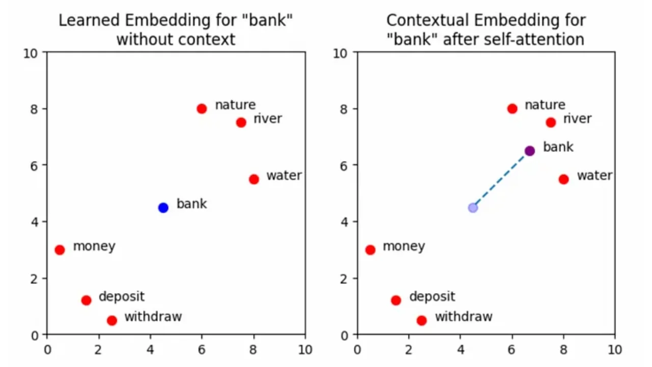
The attention mechanism is the key component in transformers that is largely responsible for their success. Attention is the method by which the model gives context to values in the input and output sequences. For example, the word bank can mean both a building which stores money and a grass verge beside a river. The sentence I withdrew money from the bank. has two key words which provide the context we need to understand the sentence: withdrew and money. Similarly, the sentence We sat on the bank and started fishing. gives context through the word fishing. Transformers use two kinds of attention:
- self-attention - where the model determines how words in the input sequence should attend to which other words in the input sequence in order to derive context
- cross-attention - where the model determines how words in the output sequence should attend to words in the input sequence in order to derive context
Decoder:
In the first decoder time step, the decoder receives the encoded input sequence and produces one output token. The encoded input is then passed back into the decoder alongside the first output token for the next time step. This process repeats iteratively until the decoder produces a stop token. The tokens are then mapped back into natural language words to produce the final response of the model.
![Transformer architecture diagram [2]](https://cms.staas.io/wp-content/uploads/2024/05/Transformer-architecture-diagram-2.webp)
Transformer architecture diagram [2].
2.4 Evolutionary Tree of LLMs
After the release of “Attention is All You Need”, a wave of research began improve and refine the attention-centric design of the transformer. 2018 saw the release of two revolutionary models which can now be considered the first modern LLMs: GPT and BERT. GPT, or Generative Pre-Trained Transformer (ancestor of the popular ChatGPT) was published by OpenAI in June 2018 in their paper “Improving Language Understanding by Generative Pre-Training” [13]. GPT uses a decoder-only architecture, meaning that the model ignores the encoder portion of the original transformer design. Four months later in October 2018, Google released their model BERT, or Bidirectional Encoder Representations from Transformers, in their paper “BERT: Pre-training of Deep Bidirectional Transformers for Language Understanding” [14]. Unlike GPT, BERT is an encoder-only model, ignoring the decoder portion of the transformer. Since then, there have been many new takes on the transformer design, producing more and more architectures every year. Below shows an image of the LLM “evolutionary tree”, highlighting some of the more notable models that have been released over the last few years. Each of which have been created with unique architectures and pre-training objectives. but largely fit into the categories: encoder-only, decoder-only, and encoder-decoder architectures. Notably, the decoder-only branch of the tree is more heavily populated than the encoder-only and encoder-decoder branches combined. This may due in part to the prevalence of autoregressive language modelling objectives, and tasks that prioritise generating coherent and contextually rich output sequences. These ideas are developed further in later articles.
![Evolutionary Tree of Large Language Models [1]](https://cms.staas.io/wp-content/uploads/2024/05/Evolutionary-Tree-of-Large-Language-Models-1.webp)
Evolutionary Tree of Large Language Models [1].
Conclusion
This article took a look at the history of language models, stretching back from cold war translation efforts, right through to the cutting-edge transformer-based models of today. The goal in doing so, was to motivate the upcoming articles in this series, which break down the inner workings of some of the most important models in the history of NLP. An appreciation for the conditions that transformers were created in help build an understanding for the design decisions that got us to where we are today. Future articles tackle key mechanisms that allow these models to work, such as self-attention, so read on if you are interested in discovering more!
Further Reading
[1] Evolutionary Tree of Large Language Models — [GitHub]
[2] Attention is All You Need — [ArXiv]
[3] An Image is Worth 16x16 Words: Transformers for Image Recognition at Scale — [ArXiv]
[4] iTransformer: Inverted Transformers Are Effective for Time Series Forecasting — [ArXiv]
[5] Machine Translation through the ages: From the cold war to deep learning — [2M Languages]
[6] Stanford CS224N NLP with Deep Learning | Winter 2021 | Lecture 7 — Translation, Seq2Seq, Attention — [YouTube]
[7] Recurrent Continuous Translation Models — [ACL Anthology]
[8] Learning Phrase Representations using RNN Encoder-Decoder for Statistical Machine Translation [ACL Anthology]
[9] Sequence to Sequence Learning with Neural Networks — [ACL Anthology]
[10] History and Frontier of the Neural Machine Translation — [SyncedReview]
[11] LONG SHORT-TERM MEMORY — [Johannes Kepler University]
[12] Transformer Language Models without Positional Encodings Still Learn Positional Information — [ArXiv]
[13] Improving Language Understanding by Generative Pre-Training — [OpenAI]
[14] BERT: Pre-training of Deep Bidirectional Transformers for Language Understanding — [ArXiv]
Source: Bradney Smith
