Word Embeddings with word2vec from Scratch in Python
Converting words into vectors with Python! Explaining Google’s word2vec models by building them from scratch. Part 2 in the "LLMs from Scratch" series - a complete guide to understanding and building Large Language Models.
Part 2 in the “LLMs from Scratch” series - a complete guide to understanding and building Large Language Models. If you are interested in learning more about how these models work I encourage you to read:
- Prelude: A Brief History of Large Language Models
- Part 1: Tokenization — A Complete Guide
- Part 2: Word Embeddings with word2vec from Scratch in Python (Current article)
- Part 3: Self-Attention Explained with Code
- Part 4: A Complete Guide to BERT with Code
Introduction
Word Embedding is the process of taking a word and creating a vector representation in N-dimensional space. As a simple example, you could imagine each word having a three-dimensional representation, and then plotting the words in 3D space using these numbers as coordinates. The goal here is to come up an algorithm to produce the coordinates for each word (called embeddings), such that similar words are geographically near in vector space, and dissimilar words are distant in vector space. Word embeddings bridge the barrier between natural language and machine language, and so the need for high quality vector representations is difficult to understate. To demonstrate the concept of word embedding, this article will look at word2vec — a family of algorithms proposed by Google in 2013. These models generate word vectors for millions of unique words across multiple languages. We will break down why the idea of representing words as vectors is important, and how the word2vec algorithms work using the Skip-Gram method (with diagrams, animations, and Python code). This will form the basis for future articles, which will discuss how Large Language Models (LLMs) produce their own embeddings by adding context to words with self-attention.
1 - Introduction to Word Embeddings
1.1 - Overview of Word Embeddings
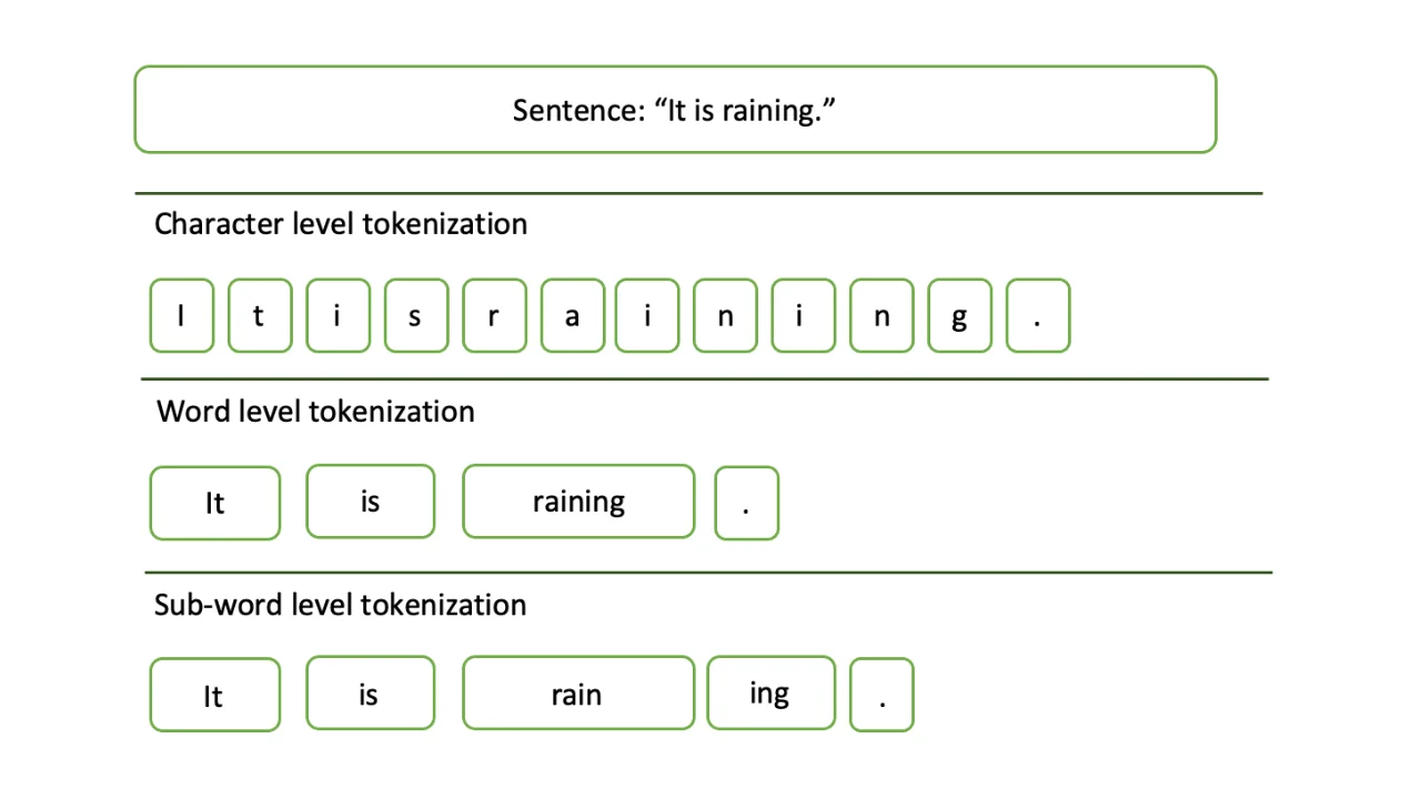
Natural Language Processing (NLP) deals with textual data, which in its raw form cannot be understood by computers. In recent times, NLP tasks have been largely handled by neural networks, such as Recurrent Neural Networks (RNNs) and transformer-based models (including many Large Language Models, LLMs). These both require vector inputs to enable linear algebra operations, and so text must first be converted into arrays of numbers. Sentences can first be split into words (or subword units) called tokens using tokenization (see LLMs from Scratch Part 1 for more on this). These tokens are then assigned an integer value called a token ID, which can be converted into a one-hot encoded vector as shown later. The process of assigning any non-numeric data, such as images and text, a numerical representation is called embedding, and so these vector representations of words are known as word embeddings. For the purposes of this article, each token will be a whole word and not part of a word. This is because the word2vec algorithm only considers entire words. In the future articles, we will look at how subword tokens are used to generate embedding vectors, such as BERT using tokens produced by WordPiece.
1.2 - Denotational vs Distributional Semantics
Before embedding words as vectors, it is important to consider what meaning is trying to be encoded. Most linguists think about meaning as being the representation of an idea by a word or group of words. This is called denotational semantics, and is just one way to define the meaning of words. For NLP, it is often more helpful to think of the meaning of a word as being determined by the words that frequently co-occur (i.e. words that often appear before or after the word). This is a concept called distributional semantics [1], and is best summed-up by British Linguist J.R.Firth in his quote [2]: "You shall know a word by the company it keeps."
Distributional semantics forms the basis of modern word embeddings, and has fundamentally changed the way we approach NLP tasks.
1.3 - Localist Word Embeddings
Prior to 2013, word embeddings were often created using one-hot encoding. This method for producing vector representations is very simple: for each word construct a vector with 0s in every element, except at the position equal to the token ID which should be filled with a 1. This creates a unique vector for each word, where the position of the 1 indicates which word is being encoded (hence the name ‘one-hot’). Because of this, one-hot vectors are called localist representations, as all the information that represents the word is restricted to a single element.
For example, consider a model that produces vectors to encode the following five words: cat, kitten, dog, puppy, and mouse. The collection of words a model can encode is called the vocabulary, and number of words in the vocabulary is called the vocabulary size. As shown below, the vocabulary size dictates the dimensions of the vectors a one-hot model will produce:
cat: [1, 0, 0, 0, 0]dog: [0, 1, 0, 0, 0]kitten: [0, 0, 1, 0, 0]mouse: [0, 0, 0, 1, 0]puppy: [0, 0, 0, 0, 1]
The vocabulary is usually ordered alphabetically, and so the order of the encodings will follow these alphabetised words. From this small example you can see that the number of elements in the vector is tied to the vocabulary size. For a model to be able to embed a vocabulary made up of 100,000 unique words, every embedding would require 100,000 elements.
Note: Another technique to create word embeddings prior to 2013 was to construct co-occurrence matrices, which are not covered in this article. If you are interested in reading more about the history of word embeddings, I would recommend Aylien’s blog post on the topic [3].
def create_vocabulary(training_data):
    """ Return a sorted list of words by tokenizing training data."""
    all_words = ' '.join(training_data).lower()
    all_words = all_words.replace('.', '')
    all_words = all_words.split(' ')
    vocab = list(set(all_words))
    vocab.sort()
    return vocab

def one_hot(word, vocab, vocab_size):
    """ Return a one-hot encoded vector for a word."""
    one_hot = [0]*vocab_size
    pos = vocab.index(word)
    one_hot[pos] = 1
    one_hot = np.array(one_hot)
    return one_hot

def create_vector_word_map(vocab, vocab_size):
    """ Return a dictionary map to convert one-hot vectors back into words."""
    vec_to_word = {str(one_hot(word, vocab, vocab_size)): word \
                      for word in vocab}
    return vec_to_word

# Create some training data
training_data = ['cat kitten dog puppy mouse']
vocab = create_vocabulary(training_data)
vocab_size = len(vocab)

# Print the one-hot encoding for each word
for word in vocab:
    print(f'{word}:{" "*(6-len(word))} {one_hot(word, vocab, vocab_size)}')
cat: [1 0 0 0 0]
dog: [0 1 0 0 0]
kitten: [0 0 1 0 0]
mouse: [0 0 0 1 0]
puppy: [0 0 0 0 1]1.4 - Limitations of One-Hot Encoding
Vectors produced by one-hot encoding have some limitations which have been addressed by the more complex vector representations discussed later in this article. The two main limitations are:
The embedding vectors have too many dimensions:
- The vocabulary size of language models can be very large; English for example uses hundreds of thousands of words. To accurately capture and represent all these words, a one-hot encoding model must produce vectors with a number of elements equal to the vocabulary size. This produces mostly empty vectors (said to be sparse), where all the information is encoded in a single element. Due to their size, these types of word vectors do not scale very well, especially with the size of language models that are used today.
Similar words are not geographically near in vector space:
- The embedding for each word is not influenced by other words that frequently co-occur — that is, these representations are denotational in nature and not distributional. For example,
catandkittenwill be just as dissimilar ascatandbuilding. In a distributive model,catshould appear in similar contexts tokittenand so would share many co-occurring words, and hence be assigned a similar vector representation. This is a desirable trait for word vectors for a few reasons. One is that training a language model to understand synonyms becomes much faster and less computationally expensive if the word vectors are similar to begin with. Another is that you can infer information about words based on their position in vector space (such as their relationships to other words), which will be discussed later in this article with the class “King - Man + Woman = Queen” example. Hopefully it follows that it would be useful to come up with a model which can encode similar words with similar vectors. For a more concrete example, consider a user entering a query into a search engine. The inputsluxury cat foodandexpensive kitten treatsare written using completely different words, yet semantically are very similar. It would be useful if the vector representations for similar words were themselves similar, so that the underlying meaning of the query is captured when returning the results. In some sense, the vectors forcatandkittenshould encode the ‘catness’ of those words. This is not possible with simple one-hot encoding because the vectors are orthogonal by nature (i.e. the dot product between them is zero).
1.5 - Distributed Word Embeddings
Distributed word embeddings have been around since the early 2000s [4], but came to prominence in 2013 with the publication of two milestone papers by Mikolov et al. at Google [5–6]. Unlike localist representations, these embeddings intrinsically capture the similarities between words. The size of the vectors is also much smaller, and not tied to the vocabulary size. This allows the embeddings to scale much better to applications with hundreds of thousands of words, as is the case with LLMs. The algorithms first proposed for learning these vector representations are collectively called word2vec.
1.6 - Overview of word2Vec
word2vec is a family of algorithms that produce distributed word embeddings for use in NLP tasks. These vectors are far denser than those created using the one-hot encoding method (i.e. very few, if any, of the elements are 0), and so they can be much smaller in size. The idea is to create an N-dimensional vector space, in which similar words are geographically close to each other. Typically, these embeddings have around 300 dimensions. Once these embeddings are created, they can be written to a file and loaded into memory when needed to essentially form a lookup table at run time. When a language model is given some input text, the text is first converted into tokens. These are then converted into vectors by finding the appropriate row in the word2vec embeddings matrix. For this reason, the embeddings produced by word2vec are called static. These static embeddings form the basis for the so-called dynamic or contextual embeddings that are used in LLMs, which are made by adding context from the surrounding sentences or paragraphs to each word.
1.7 - Visualising Word Vectors
Before diving into the specifics of how these embeddings are created, it would be useful to take a look at where we are going. Below is a plot showing how 3-dimensional vectors (N=3) can be used to embed the example vocabulary given in the one-hot encoding section above. Each vector is defined using three values, so the words can be plotted in 3D space. In this 3-dimensional vector space, words that are similar (such as cat and kitten) are geographically close to each other, and words that are dissimilar (such as cat and dog) are geographically distant. This example shows three-dimensional vectors since they are easy to visualise, but the same principles hold true for higher-dimensional vectors. Hence, it is not only possible, but practical to represent word vectors using a few hundred dimensions.
# Create figure
fig = plt.figure()
ax = fig.add_subplot(projection='3d')
ax.set_title('Example Word Embeddings in 3D')

# Word embeddings
word_embeddings = [[5, 3, 1],
                   [4.5, 4.5, 0.5],
                   [1, 5, 1],
                   [1.5, 4.5, 0.5],
                   [1, 1, 5]]

# Labels for plotting
labels = ['cat', 'kitten', 'dog', 'puppy', 'mouse']

# Create plot
for we, label in list(zip(word_embeddings, labels)):
    ax.scatter(we[0], we[1], we[2], s=50)
    ax.text(we[0]+0.1, we[1]+0.1, we[2], label, size=13)
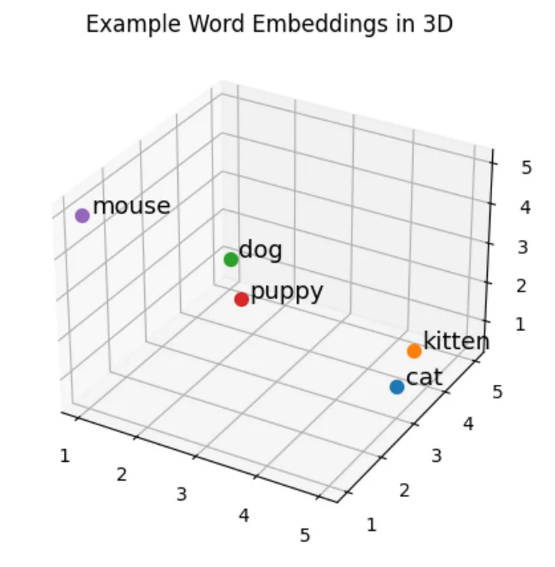
Example word embeddings (N=3) plotted in three-dimensional vector space
1.8 - The Need for High-Dimensional Vectors
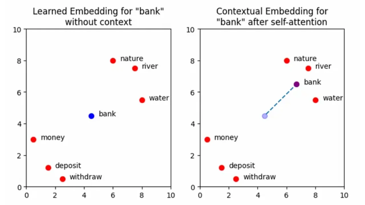
After seeing the 3D representations above, you may be wondering “why is it necessary to use 300 dimensions to represent a word when three seems to be enough?”. In our example, three dimensions is enough to show clusters of a few simple words such as (cat and kitten) and (dog and puppy). However, with a larger number of words it becomes important to represent the similarities between words in more complex ways. For example, bank is both a building which stores your money, but also the mound of dirt and grass beside a river. By using higher dimensions, the vector for bank can be geographically near the words money, loan, and debt in some dimensions and near river, water, and nature in others. Words with multiple distinct meanings are called polysemous words, and can be difficult to distinguish without the context of the whole sentence. When deciding on the number of dimensions to use for the embeddings (called the embedding dimensions), there is a trade-off between the complexity that the representation can capture and the training time for the embedding and language models.
2 - The word2vec Algorithms: Skip-Gram and CBOW
2.1 - Center Words and Outside Words
The word2vec algorithms process a sentence one word at a time, which the white paper refers to as the center word, denoted w(t). Since word2vec is a distributed model, the algorithms also consider the surrounding context words, called outside words. The number of words considered before and after the center word is determined by a hyperparameter called the window size, which is chosen by the user before training the model. For a window size of 1, the model will take 1 word before and after the center word to create the list of outside words. These are referred to mathematically as w(t-1) and w(t+1) respectively. The image below shows an example for a window size of 1, a center word of cat (highlighted in green) and outside words the and around (highlighted in red).

Center and outside words for an example sentence using word2vec
For a window size of 2, two words are taken before and after the center word (giving four words in total), and so on. If it is not possible to take any words before or after the center word, then model will simply take what is available. For example, the first the in the sentence above has no previous words w(t-1) or w(t-2). In this case with a window size of 2, the outside words will only be dog and chased. Window sizes vary based on the use-case and can be tuned to find the most appropriate value, however typical values range from 1–10 [7].
2.2 - Skip-Gram and CBOW Comparison
The word embeddings in the 3D visualisation above were hard coded to show the concept of similar words having similar vectors. In reality, these word vectors are not written by hand, but are instead learned by a word2vec (or other word embedding) model. The original papers propose two methods for learning these word vectors called Skip-Gram and Continuous Bag of Words (CBOW). These methods are very similar to each other, with both using a neural network with a single hidden layer to generate the word vectors. The difference lies in their objectives:
- Skip-Gram: Takes in a center word and predicts the outside words
- CBOW: Takes in some outside words and predicts the center word
This article will focus on explaining the Skip-Gram method in detail, but once this algorithm is understood the same principles can be easily applied to understand the CBOW method. The diagram below shows the Skip-Gram model architecture using the example sentence and center word from above, with a window size of 1.
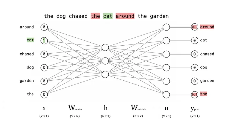
Skip-Gram architecture diagram showing an overview of a forward pass of the network
2.3 - Skip-Gram Forward Pass Overview
The diagram above gives an overview of the model architecture, but to get a more complete picture of what the model is doing, let’s take a look at each component of the diagram. Below is an explanation of a complete forward pass of the model: taking word all the way from the input layer to the output layer. This is also shown in diagram form with an animated GIF below.
Input Layer, x:
The model is trained on a corpus of words T where each t is a single token from the corpus encoded as a one-hot vector, x. This vector has a length of V (where V is equal to the vocabulary size of the model), and is inputted to the model via the input layer.
Weights Between the Input Layer and Hidden Layer, W_center:
Each node in the input layer is connected to every node in the hidden layer by N weights, where N is the number of embedding dimensions. For V input nodes, this gives a total of V ⋅ N weights which can be stored in the V × N matrix, W_center. In the example we have looked at so far, N has been set to 3 to obtain three-dimensional word embeddings that we can visualise with a scatter plot. However in real applications, N will typically be much larger. The values of the weights in W_center are initialised randomly using a Normal or uniform distribution, and iteratively improved using backpropagation as the model is trained (more on this later).
The W_center matrix is actually the output we want from the trained model, that is, it is the matrix of word embeddings for center words. The tᵗʰ row of the matrix is an N-dimensional vector that represents the tᵗʰ word in the vocabulary. After the model is trained, the W_center matrix can be extracted and saved to a file to form the lookup table of word embeddings for the model’s vocabulary.
Hidden Layer, h:
The goal of the hidden layer, h, is to use W_center as a lookup table to convert the input x into an N-dimensional word vector. This is achieved by configuring the nodes in the hidden layer to have a bias of 0 and setting the activation function to the identity function. Computationally, this means that the hidden layer is calculated by taking the dot product of the input vector, x, and the weights matrix, W_center. Since x is a one-hot encoded vector, only the tᵗʰ element is non-zero. As a result, the dot product x ⋅ W_center contains only the tᵗʰ row of W_center, giving the lookup table behaviour we wanted.
Weights between the Hidden Layer and Output Layer, W_outside:
Now that the network has an N-dimensional word vector for the input, it can perform further processing to form a prediction for the outside words. To do this, the dot product is taken between the hidden layer, h, and the second weights matrix, W_outside. This matrix stores the word embeddings for each word in the vocabulary when they act as a context word, rather than as a center word. Practically, this matrix is not often used other than to train the model to produce the optimum values for W_center. There is some discussion in literature for using this matrix for word embeddings instead of W_center, but the results don’t seem to hold up as well [1].
Note: W_outside has dimensions N × V, which you might notice is the transpose of W_center. This is solely to make the dot product with h simpler. This is personal preference — many sources define W_outside to have dimensions V × N and explicitly use the transpose to form the dot product with h. To account for the shape change in our model, the word embeddings in W_outside are stored as columns instead of rows (unlike W_center).
Output Layer, u, and Softmax Values, y_pred:
The output layer, u, stores the raw outputs of the network (called logits) in a V-dimensional vector. Each element of u corresponds to the “probability” of the word being an outside word for the given center word. To ensure these “probabilities” sum to 1, the softmax function is applied to produce the final predictions vector, y_pred. If you are familiar with the argmax function, this cannot be used here since it does not have a smooth derivative and so is incompatible with the backpropagation algorithm that is employed later.
Note: strictly speaking, for these values to be true probabilities the network would need to be perfectly calibrated (which it probably is not). Neural networks tend to be overconfident in their estimates, and so can claim that an output has a 90% probability when in reality the network is only correct 50% of the time. When this happens the network is said to be uncalibrated. This is a general problem for all neural networks and is not specific to the Skip-Gram architecture. Just note that for the purpose of this explanation, the term probability is not completely incorrect, but it is not 100% accurate either. However, the topic of uncertainty quantification can be saved for a later day.
Consider a case where the center word is cat and the values of y_pred are [0.4, 0.05, 0.1, 0.05, 0.3, 0.1]. This implies that around and garden are the most likely outside words since they produce the highest softmax scores. We were hoping to see around and the as the outside words, and so we need some method of quantifying this mistake so that the network can learn. We also want to repeat this for every center word in the training data, and apply the appropriate corrections to word embedding matrices W_center and W_outside. These quantifications and corrections take place in the backwards pass.

Animated GIF of a forward pass of the Skip-Gram word embedding model
2.4 - Forward Pass — Encode the Center Words and Outside Words
To begin training the model, the training data must be split into words (tokens) using Tokenization. For this example, the text has simply been split on spaces and converted to lowercase with punctuation removed using regular expressions. The set of unique tokens can be ordered alphabetically to form a vocabulary for the one-hot encoding model. Finally, for each center word in the text, the outside words can be found and converted to one-hot vectors along with the center word and stored in a list. This list of center words and corresponding outside words will be used to train the model.
import re

WINDOW_SIZE = 2

def encode_training_data(training_data, vocab_size, window_size):
    """ Encode the center and outside words as one-hot vectors."""

    encoded_training_data = []

    for sentence in training_data:

        # Tokenize the sentence
        tokens = re.sub(r'[^\w\s]', '', sentence).lower().split(' ')

        # Encode each center word and its surrounding context words
        for word_pos, word in enumerate(tokens):
            center_word = one_hot(word, vocab, vocab_size)

            outside_words = []
            for outside_pos in range(word_pos-window_size,
                                     word_pos+window_size+1):
                if (outside_pos >= 0) and (outside_pos < len(tokens)) \
                and (outside_pos != word_pos):
                    outside_words.append(one_hot(tokens[outside_pos],
                                                 vocab,
                                                 vocab_size))

            encoded_training_data.append([center_word, outside_words])

    return encoded_training_data

def print_training_encodings(encoded_training_data, vocab, vec_to_word):
    """ Print the encodings for each (center word - outside words) set."""

    max_len = len(max(vocab, key=len))

    for num, (cw_vector, ow_vectors) in enumerate(encoded_training_data):

        cw = vec_to_word[str(cw_vector)]
        ow = vec_to_word[str(ow_vectors[0])]

        print(f'Center Word #{num}: {cw}{" "*(max_len-len(cw))} {cw_vector}')
        print(f'Outside Words:  {ow}{" "*(max_len-len(ow))} {ow_vectors[0]}')

        if len(ow_vectors) > 1:
            for i in range(len(ow_vectors)-1):

                outside_word = vec_to_word[str(ow_vectors[i+1])]
                print(f'{" "*16}{ow}{" "*(max_len-len(ow))} {ow_vectors[i+1]}')

        print()

# Create training data
training_data = ['The dog chased the cat around the garden.']

# Encode training data
vocab = create_vocabulary(training_data)
vocab_size = len(vocab)
vec_to_word = create_vector_word_map(vocab, vocab_size)
encoded_training_data = encode_training_data(training_data,
                                             vocab_size,
                                             window_size=WINDOW_SIZE)

# Print out results
print_training_encodings(encoded_training_data, vocab, vec_to_word)
Center Word #0: the [0 0 0 0 0 1]
Outside Words: dog [0 0 0 1 0 0]
chased [0 0 1 0 0 0]
Center Word #1: dog [0 0 0 1 0 0]
Outside Words: the [0 0 0 0 0 1]
chased [0 0 1 0 0 0]
the [0 0 0 0 0 1]
Center Word #2: chased [0 0 1 0 0 0]
Outside Words: the [0 0 0 0 0 1]
dog [0 0 0 1 0 0]
the [0 0 0 0 0 1]
cat [0 1 0 0 0 0]
Center Word #3: the [0 0 0 0 0 1]
Outside Words: dog [0 0 0 1 0 0]
chased [0 0 1 0 0 0]
cat [0 1 0 0 0 0]
around [1 0 0 0 0 0]
Center Word #4: cat [0 1 0 0 0 0]
Outside Words: chased [0 0 1 0 0 0]
the [0 0 0 0 0 1]
around [1 0 0 0 0 0]
the [0 0 0 0 0 1]
Center Word #5: around [1 0 0 0 0 0]
Outside Words: the [0 0 0 0 0 1]
cat [0 1 0 0 0 0]
the [0 0 0 0 0 1]
garden [0 0 0 0 1 0]
Center Word #6: the [0 0 0 0 0 1]
Outside Words: cat [0 1 0 0 0 0]
around [1 0 0 0 0 0]
garden [0 0 0 0 1 0]
Center Word #7: garden [0 0 0 0 1 0]
Outside Words: around [1 0 0 0 0 0]
the [0 0 0 0 0 1]2.5 - Forward Pass — Calculate the Hidden Layer Vector
Once the center words and their respective outside words are encoded, the center words can be fed into the network one at a time to complete their forward pass. The hidden layer is simply the tᵗʰ row of the W_center matrix because all other rows in the x vector are 0. The animation below shows the hidden layer vector, h, for each center word in the vocabulary.
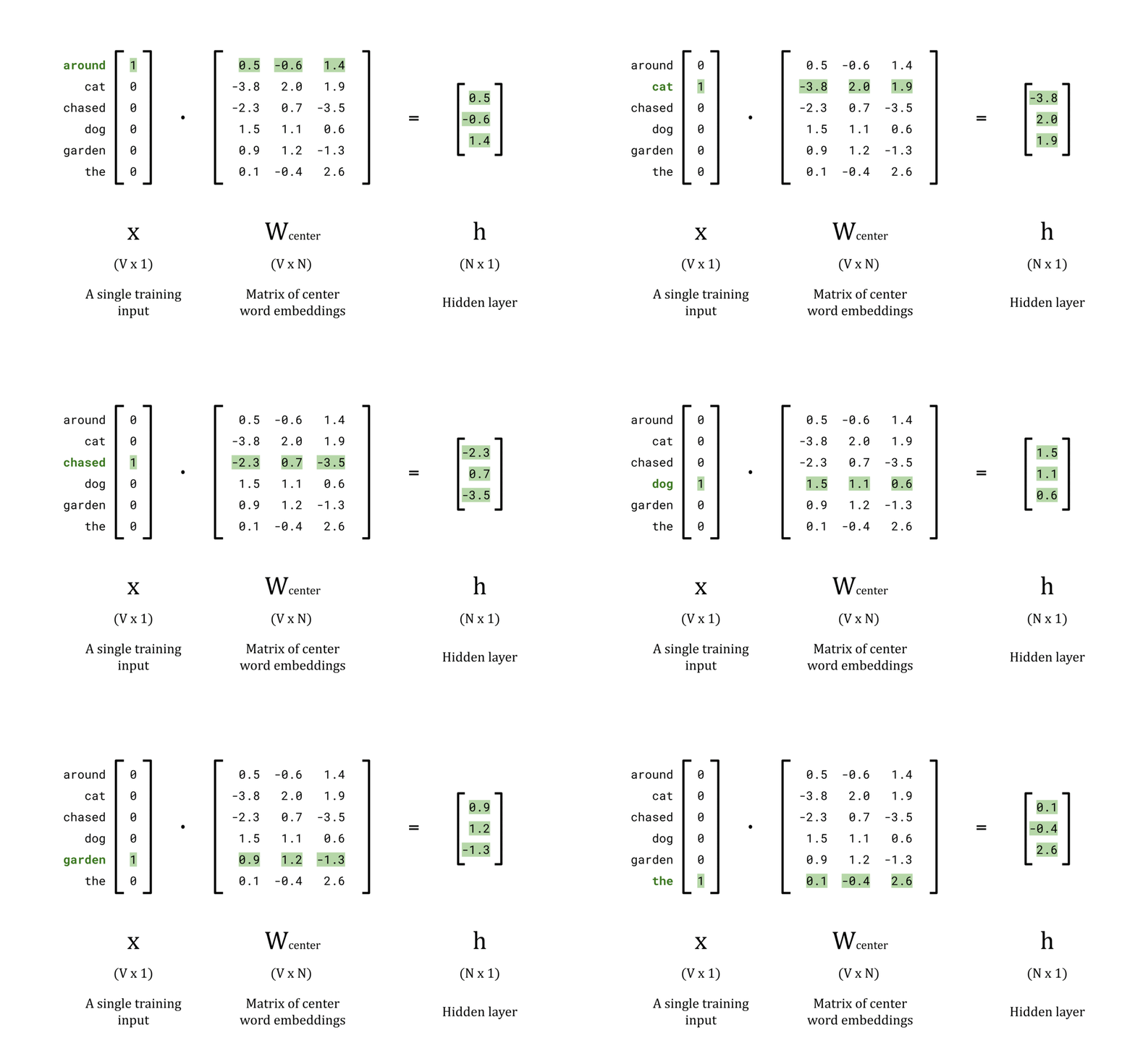
Animated GIF showing the calculation of the hidden layer for a forward pass
EMBEDDING_DIM = 3

# Calculate the hidden layer vector
x = encoded_training_data[0][0]
w_center = np.random.rand(vocab_size, EMBEDDING_DIM)
h = np.dot(x, w_center)

# Print the results
print(f'Center word, w(t): {vec_to_word[str(x)]}\n')
print(f'Input vector, x:   {x}\n')
print(f'W_center: \n\n{w_center}\n')
print(f'Hidden layer, h:   {h}\n')
Center word, w(t): the
Input vector, x: [0 0 0 0 0 1]
W_center:
[[0.97059646 0.05009912 0.04528659]
[0.62298807 0.05217879 0.95444055]
[0.08574668 0.03581978 0.30344068]
[0.61045573 0.26872761 0.32452861]
[0.87073368 0.18103158 0.5336525 ]
[0.86663298 0.41447729 0.58625039]]
Hidden layer, h: [0.86663298 0.41447729 0.58625039]2.6 - Forward Pass — Calculate the Network Outputs, u
The next stage of the forward pass is to compute the dot product of the hidden layer vector, h, and the weight matrix of outside words, W_outside. This will produce the raw network outputs, u, which is a V dimensional vector of logits. These will be converted to “probability” values by the softmax function in the next stage.
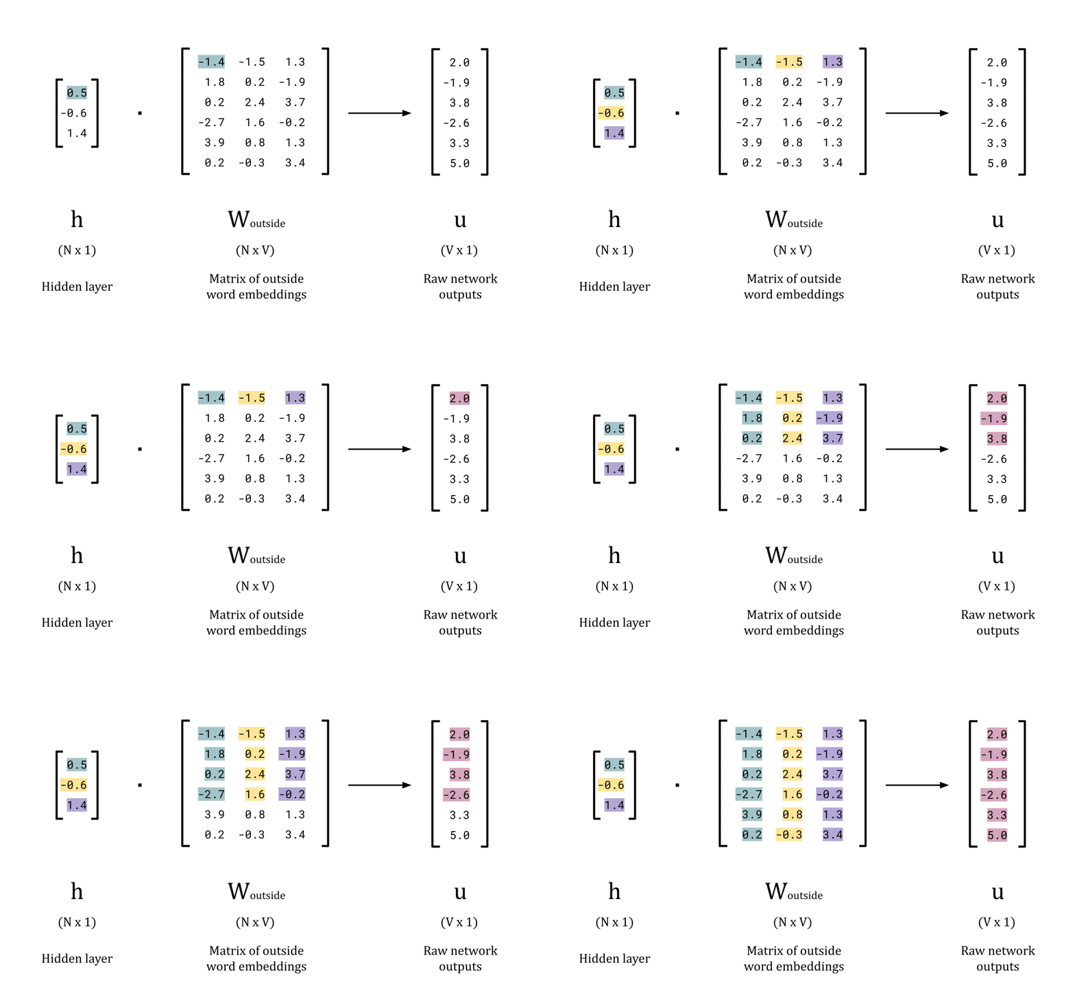
Animated GIF showing the calculation of the logits for a forward pass
# Calculate the raw network outputs
w_outside = np.random.rand(EMBEDDING_DIM, vocab_size)
u = np.dot(h, w_outside)

# Print the results
print(f'Hidden layer, h:   {h}\n')
print(f'W_outside: \n\n{w_outside}\n')
print(f'Raw network outputs (logits), u:   {u}\n')
Hidden layer, h: [0.86663298 0.41447729 0.58625039]
W_outside:
[[0.11052363 0.28507393 0.35390072 0.41468025 0.79666595 0.56870707]
[0.18695443 0.51800033 0.77617465 0.05332514 0.81199024 0.16522743]
[0.81727698 0.69201976 0.07326851 0.70986966 0.89684757 0.62262952]]
Raw network outputs (logits), u: [0.65240074 0.8674507 0.67136249
0.79763901 1.55274574 0.92636012]2.7 - Forward Pass — Calculate the Predictions, y_pred
To complete the forward pass, the raw outputs vector, u, will be converted elementwise to give a set of scores using the softmax function. The value of each element corresponds to a “probability” of a word belonging to the set out outside words for the given center word, x. For a window size of 1, the top two scores will be taken as the w(t-1) and w(t+1) predictions. For a window size of 2, the top four scores will be taken, and so on. The softmax function is given by:

Equation for the softmax function
where:
- uᵢ is an element of the raw outputs vector, u
def softmax(u):
    """ Return the softmax values for a vector u."""

    values = np.exp(u)/np.sum(np.exp(u))
    return values

def find_outside_words(y_pred, vocab, window_size):
    """ Predict outside words for a given center word from softmax outputs."""

    # Get a sorted list of softmax scores
    sorted_y_pred = y_pred.copy()
    sorted_y_pred.sort()
    sorted_y_pred = sorted_y_pred[::-1]

    # Find the outside words
    outside_words = []
    top_scores = sorted_y_pred[:window_size*2]

    for score in top_scores:
        index = np.where(y_pred == score)[0][0]
        word = vocab[index]
        outside_words.append(word)

    return outside_words

# Calculate the softmax outputs
y_pred = softmax(u)
outside_words = find_outside_words(y_pred, vocab, WINDOW_SIZE)

# Print the results
print(f'Raw network outputs (logits), u:   {u}\n')
print(f'Softmax outputs, y_pred:           {y_pred}\n')
print(f'Outside words:                     {" ".join(outside_words)}')
Raw network outputs (logits), u:   [0.65240074 0.8674507  0.67136249
                                    0.79763901 1.55274574 0.92636012]

Softmax outputs, y_pred:           [0.12208529 0.15137647 0.12442233
                                    0.14116906 0.30038498 0.16056186]

Outside words:                     garden the cat dog
2.8 - Skip-Gram Backward Pass Overview
After a forward pass, the model will produce a set of predictions for the outside words as was shown in the code cell above. The next step is to calculate the difference between what the model produced and what we hoped the model would produce (called the prediction error) for each of the outside words. After that, we then need to determine how best to change the weights in W_center and W_outside so that the difference between the model outputs and desired outputs is reduced. We can then repeat this process for more center word forward passes, to iteratively improve the model until the error is minimised. At this point the model is trained. Just as the forward pass is the process of moving forward through the network to calculate the predictions, the backward pass is the process of moving backward through the network to apply corrections to the weights.
2.9 - Backward Pass — Loss Function
To be able to improve the model, we need to establish a way to describe the performance as a function of the model parameters (in this case the weights in W_center and W_outside). Such a function is called a loss function (also called a cost function or an objective function). With a loss function in place, we can use backpropagation to determine which changes to the weights will cause an improvement in the model outputs. The loss function used in the original paper was negative log likelihood. To build up to why this particular function was chosen, let’s first examine the likelihood function, which is given by:

Equation for the likelihood function
where:
- θ is all the parameters of the model, in this case all the individual weights in the W_center and W_outside matrices
- T is the collection of all the words in the corpus
- m is the window size
This function calculates a score for the model by going through a few steps:
- Start with the first word, w_t, in the corpus, T.
- For a window size, m, calculate the probability of the surrounding words being outside words according to your model (i.e. using the current weight parameters via a forward pass). The probabilities P(w_t+j | w_t; θ) are simply the softmax scores calculated in the final layer of the network.
- Multiply these probability scores together.
- Repeat this process for each word t in the corpus, multiplying the results together each time.
- The final result is a likelihood score, that should be high when the model performing well (predicting that the actual outside words should be outside words), and low when the model is performing poorly (believing the actual outside words should not be outside words).
Optimising this function in its current state forms a maximisation problem, where want to achieve a high likelihood score. In machine learning however, it is common to frame problems as minimisation tasks, and so a negative sign can be placed in front of the entire expression arbitrarily to convert this to a minimisation problem.
To convert this loss function to the negative log likelihood function as stated in the beginning, we can take the log of both sides. This is a useful trick for computation because we can exploit the laws of logarithms. Recalling the property of logs such that log(A × B) = log(A) + log(B), when can convert the product sign into a summation sign in the equations. This performs very well on machines optimised for basic arithmetic such as addition using for loops. To round the equation off, it is also common to see a factor of 1/T in front to give a normalising effect. This is not required, but can be useful when comparing model performances since the loss is no longer dependent on the size of the corpus. In this form, the loss function is given the symbol J(θ) and is written as:

Equation for the negative log likelihood (cross entropy) loss function
Finally, there is one further modification we can make to this loss function. In its current form, the equation requires the calculation of the probability values for all T center words, which could be billions of words. To increase computational speed, the loss of each center word t can be calculated instead. This will allow us to use Stochastic Gradient Descent in the next step, and update the weights after each center word. Now, the final equation looks like:

Equation for a variant of the negative log likelihood loss function for use with stochastic gradient descent
This loss function is also called the cross entropy, and is often used when training a model to predict categorical outputs encoded as one-hot vectors [8].
def calculate_loss(outside_words, y_pred):
    """ Calculate the loss using negative log likelihood."""
    # Combine the one-hot outside word vectors into a single vector with 1s for
    # each outside word and 0s for all other words
    combined_outside_words = np.sum(outside_words, axis=0)

    # Multiply by y_pred element-wise to get the components of y_pred that are
    # inside the window
    components = np.multiply(combined_outside_words, y_pred)

    # Find the indexes of the non-zero values in the components vector and
    # remove them to prevent taking log(0) in the next step
    non_zero_idx = np.where(components != 0)[0]
    non_zero_components = components[non_zero_idx]

    # Take the log of the non-zero values
    log_components = np.log(non_zero_components)

    # Sum the log of the
    loss = -np.sum(log_components)

    return loss
2.10 - Backward Pass — Backpropagation
This article assumes you are already familiar with gradient descent and backpropagation, but as a refresher:
- Gradient Descent: an optimisation algorithm to iteratively improve the performance of a model by descending down the gradient of an error surface, and find locally/globally optimum parameter values to minimise a loss function.
- Backpropagation: a fast algorithm to compute the gradient of a loss function, needed when implementing gradient descent in neural networks.
In our case, stochastic gradient descent combined with backpropagation can be used to minimise the negative log likelihood loss function, thus improving the performance of the model to predict the outside words for each given center word. The key equations for gradient descent in this application are:
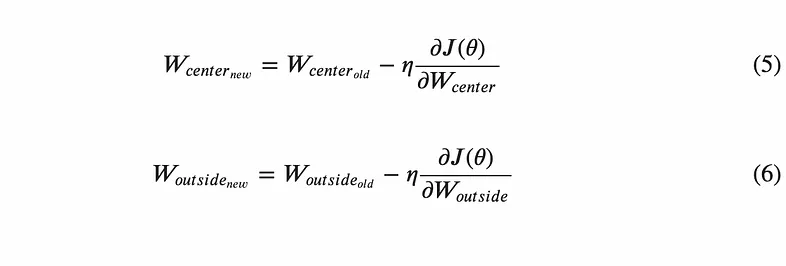
Equations for updating the weight matrices using gradient descent
where:
- η is the learning rate, a factor that encourages convergence to an optimum solution in gradient descent.
Backpropagation will be used to calculate partial derivative of J(θ) with respective to W_center and also the partial derivative of J(θ) with respective to W_outside. The results of taking the partial differentials of equation (4) with respect to W_center and W_outside can be shown to give:
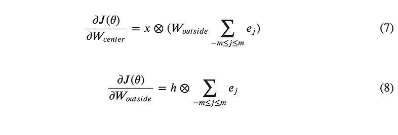
Equations for calculating the gradient of the loss function with backpropagation, which can then be used in (5) and (6) to perform gradient descent
where:

Equation for the definition of e_j, the difference between the vectors y_true_j (the jth outside word in the window) and y_pred (the network prediction)
and:
- ⊗ is the outer product, which is used to create a matrix from two vectors.
- e is the prediction error — the difference between the desired values of the network and the actual output values. For four outside words (i.e. a window size of
2), j will range from1to4, and so there will be four e vectors: e_1 to e_4.
2.11 - Skip-Gram Summary
This section has covered the inner workings of the Skip-Gram algorithm in some detail, but zooming out will allow us to see the bigger picture of what the algorithm is doing. When view holistically, the algorithm is fairly straightforward. Here is a summary of the steps:
Randomly initialise the W_center and W_outside matrices.
Take in a one-hot encoded vector for a center word, x.
Calculate the hidden layer vector by taking the dot product of x and W_center.
Calculate the raw network outputs, u, (logits) by taking the dot product of h and W_outside.
Convert the logits to “probability” values using the softmax function.
Calculate the prediction error between the softmax outputs and every one-hot encoded outside word vector in the window.
Calculate the loss (used later in step 9).
Apply equations (7) and (8) to update the weights in W_center and W_output.
Repeat steps 2–7 for each center word in the corpus.
Repeat step 8 for each epoch (iteration using the same training data again) until the loss has plateaued.
The network is now trained, and the W_center matrix can be written to a file and loaded into memory when needed to be used as a lookup table for word embeddings.
2.12 - Skip-Gram Python Implementation
Now that the basis for the algorithm has been established, we can create a custom Python implementation from scratch. It is useful to give the model some additional data to train on, so below is a list of some sentences we can use:
The dog chased the cat around the garden
The cat drank some waterThe dog ate some foodThe cat ate the mouse
import matplotlib.pyplot as plt
import numpy as np
import re

class word2vec:
    """ An implementation of the word2vec Skip-Gram algorithm.

    Attributes:
        embedding_dim (int): The number of dimensions in the output word
            embeddings.
        window_size (int): The number of outside words to consider either side
            of a center word.
        epochs (int): The number of epochs to use in training.
        learning_rate (float): The learning rate used for gradient descent to
            iteratively improve the weight matrices. Smaller values (~0.01) are
            generally preferred.
        embeddings (np.array[np.array]): The matrix of static word embeddings
            produced by the model.
        encoded_training_data (np.array[np.array]): A collection of center
            words and their corresponding outside words encoded as one-hot
            vectors.
        losses (list[int]): The loss for each epoch of the model's training.
            Can be used to plot the decrease in the loss over training.
        training_data (list[str]): A list of strings of raw text, which is
            converted to encoded_training_data and used to train the model.
        vec_to_word (dict): A dictionary which maps a string version of the
            one-hot vector to a word string.
        vocab (list): An alphabetised list of all the unique words in the
            training data.
        vocab_size (int): The number of unique words in the training data.
    """

    def __init__(self, embedding_dim, window_size, epochs, learning_rate):
        self.embedding_dim = embedding_dim
        self.window_size = window_size
        self.epochs = epochs
        self.learning_rate = learning_rate

        self.embeddings = None
        self.encoded_training_data = None
        self.losses = []
        self.training_data = None
        self.vec_to_word = None
        self.vocab = None
        self.vocab_size = None

    def calculate_loss(self, outside_words, y_pred):
        """ Calculate the loss.

        Calculate the loss according to the negative log likelihood function.
        This requires taking the sum of the log P(w_{t+j}|w_t) values (log of
        the softmax outputs, y_pred). To do this, first combine all the one-hot
        encoded outside word vectors into a single vector called
        combined_outside_words. For example, if two outside words have vectors
        [0 1 0 0 0 0] and[0 0 0 0 1 0], the combined_outside_words vector will
        be [0 1 0 0 1 0]. Next multiply this new vector with the softmax
        outputs, y_pred, to obtain the softmax values for the outside words -
        store the result in a vector called components. The components vector
        will have some elements with a value of 0, and so these should be
        removed before taking the elementwise log of the vector. After removing
        and taking the log of the remaining elements, sum the log values to
        give the loss and return the value.

        Args:
            outside_words (np.array[np.arrays]): An array of one-hot encoded
                vectors for each outside word.
            y_pred (np.array): An array of softmax outputs from the network for
              a given center word.

        Returns:
            loss (float): The loss of the network for the input center word.

        """
        # Combine the one-hot outside word vectors into a single vector with 1s
        # for each outside word and 0s for all other words
        combined_outside_words = np.sum(outside_words, axis=0)

        # Multiply by y_pred element-wise to get the components of y_pred that
        # are inside the window
        components = np.multiply(combined_outside_words, y_pred)

        # Find the indexes of the non-zero values in the components vector and
        # remove them to
        # prevent taking log(0) in the next step
        non_zero_idx = np.where(components != 0)[0]
        non_zero_components = components[non_zero_idx]

        # Take the log of the non-zero values
        log_components = np.log(non_zero_components)

        # Sum the log of the
        loss = -np.sum(log_components)

        return loss

    def create_vec_to_word_map(self):
        """ Return a map to convert one-hot vectors back into words."""
        self.vec_to_word = {str(one_hot(word, self.vocab, self.vocab_size)): \
                            word for word in self.vocab}

    def create_vocabulary(self):
        """ Return a sorted list of words by tokenizing training data."""
        all_words = ' '.join(training_data).lower()
        all_words = all_words.replace('.', '')
        all_words = all_words.split(' ')
        self.vocab = list(set(all_words))
        self.vocab.sort()
        self.vocab_size = len(self.vocab)

    def encode_training_data(self):
        """ Encode the center and outside words as one-hot vectors."""

        self.encoded_training_data = []

        for sentence in training_data:

            # Tokenize the sentence
            tokens = re.sub(r'[^\w\s]', '', sentence).lower().split(' ')

            # Encode each center word and its surrounding context words
            for word_pos, word in enumerate(tokens):
                center_word = self.one_hot(word)

                outside_words = []
                for outside_pos in range(word_pos-self.window_size,
                                         word_pos+self.window_size+1):

                    if (outside_pos >= 0) and (outside_pos < len(tokens)) \
                    and (outside_pos != word_pos):

                        outside_words.append(self.one_hot(tokens[outside_pos]))

                self.encoded_training_data.append([center_word, outside_words])

    def one_hot(self, word):
        """ Return a one-hot encoded vector for a word.

        Args:
            word (str): A word from the training data.

        Returns:
            one_hot (np.array): A one-hot encoded vector representation of the
                input word.
        """
        one_hot = [0]*self.vocab_size
        pos = self.vocab.index(word)
        one_hot[pos] = 1
        one_hot = np.array(one_hot)
        return one_hot

    def softmax(self, u):
        """ Return the softmax values for a vector u.

        Args:
            u (np.array): A vector of raw network outputs (logits).

        Returns:
            values (np.array): A vector of softmax values for the input, u.
        """
        values = np.exp(u)/np.sum(np.exp(u))
        return values

    def train(self, training_data):
        """ Take in raw text and produce a matrix of word embeddings.

        From the raw text in training_data, create an alphabetised vocabulary
        of unique words and encode each center word and its corresponding
        outside words as one-hot vectors. Initialise the weights matrices
        W_center and W_outside that store the connections between the layers in
        the network. For each center word in the encoded training data,
        compute a forward, calculate the loss, and compute a backward pass.
        Print the loss for each epoch and repeat until every epoch has been
        completed. Store the final embeddings in the self.embeddings attribute.

        Args:
            training_data (list[str]): A list of strings of raw text, which is
                converted to encoded_training_data and used to train the model.

        Returns:
            None.
        """
        self.create_vocabulary()
        self.encode_training_data()

        # Initialise the connections between layers
        W_center = np.random.rand(self.vocab_size, EMBEDDING_DIM)
        W_outside = np.random.rand(EMBEDDING_DIM, self.vocab_size)

        for epoch_num in range(self.epochs):

            loss = 0

            for x, outside_words in self.encoded_training_data:

                # Forward pass
                h = np.dot(x, W_center)
                u = np.dot(h, W_outside)
                y_pred = self.softmax(u)

                # Calculate the loss
                loss += self.calculate_loss(outside_words, y_pred)

                # Backward pass
                e = np.sum([y_pred - ow for ow in outside_words], axis=0)
                grad_W_outside = np.outer(h, e)
                grad_W_center = np.outer(x, np.dot(W_outside, e))
                W_outside = W_outside - (self.learning_rate * grad_W_outside)
                W_center = W_center - (self.learning_rate * grad_W_center)

            self.losses.append(loss)
            print(f'Epoch: {epoch_num+1}    Loss: {loss}')

        self.embeddings = W_center

EMBEDDING_DIM = 3
WINDOW_SIZE = 2
EPOCHS = 1000
LEARNING_RATE = 0.01

# Create training data
training_data = ['The dog chased the cat around the garden.',
                 'The cat drank some water.',
                 'The dog ate some food.',
                 'The cat ate the mouse.']

# Instantiate the model
w2v = word2vec(embedding_dim = EMBEDDING_DIM,
               window_size = WINDOW_SIZE,
               epochs = EPOCHS,
               learning_rate = LEARNING_RATE)

# Train the model
w2v.train(training_data)
Epoch: 1 Loss: 155.544040703127
Epoch: 2 Loss: 152.86073600205606
Epoch: 3 Loss: 150.56449634379754
...
Epoch: 998 Loss: 99.39131539280359
Epoch: 999 Loss: 99.38810367351859
Epoch: 1000 Loss: 99.384898883075922.13 - Plot the Word Embeddings
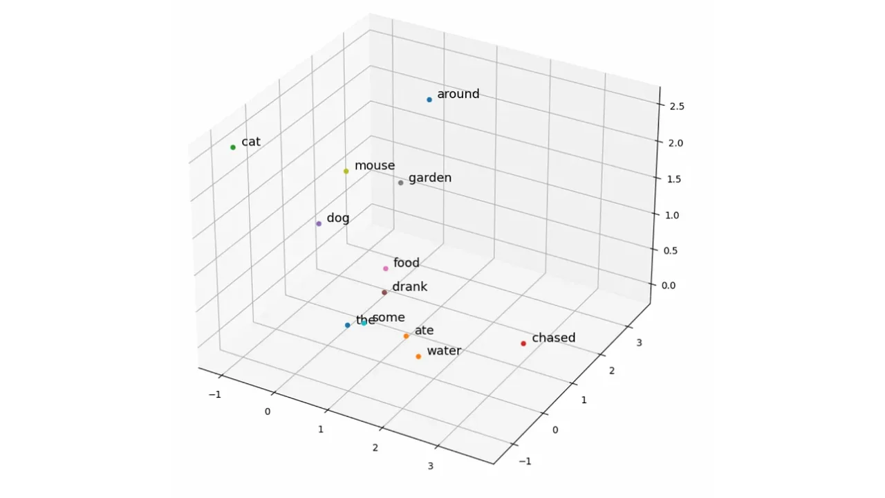
Despite the limited corpus size the model has produced some fairly good results. For example, since food and water co-occur with eat and drink in the training data, they are geographically near in vector space. The words cat, dog, and mouse also occupy a similar region of the vector space. In this case, the “animalness” of these words is likely not what is being captured, but rather their function in the sentence as nouns — hence why garden is also in a similar region of the space. However, with many more words in the training data (e.g. billions), the hope is that this “animalness” as well as many other properties will be encoded.
# Plot the word embeddings
fig = plt.figure(figsize=(10,10))
ax = fig.add_subplot(projection='3d')

for i, (x,y,z) in enumerate(w2v.embeddings):
    ax.scatter(x,y,z)
    ax.text(x+0.1, y+0.1, z, w2v.vocab[i], size=13)
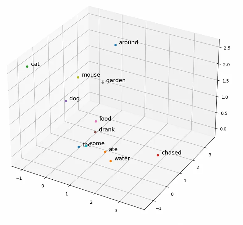
Plot of word embeddings created with Python implementation of the Skip-Gram method
2.14 - Visualising the Decrease in Loss
The loss gradually improves with each epoch as the network trains. Determining how many epochs to use can be very much a trial and error process. A good approach is to plot the loss curve as the network trains and stop when the decrease in loss appears to reach an asymptote which signifies a point of diminishing returns.
# Plot the loss with each epoch
import matplotlib.pyplot as plt

fig, ax = plt.subplots(figsize=(10,5))
ax.set_title(f'Loss over {EPOCHS} Epochs')
ax.set_xlabel('Epoch')
ax.set_ylabel('Loss')

y = w2v.losses
x = list(range(EPOCHS))

ax.plot(x, y)
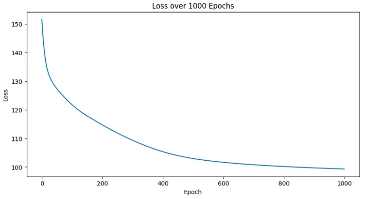
Loss curve for training a Skip-Gram model with 1000 epochs
2.15 - Training the Model on a Larger Corpus
To push the model a step further, it can be trained on a larger corpus (collection of text). Google used the entire of Wikipedia to train the original word2vec models in 2013, but this of course took several days of constant computation (even with the computational tricks they used to boost the speed of the algorithm). Here, if your computer is powerful enough, you can try training the model on the book “Emma” by Jane Austin. The copyright for this work has long expired and so the book is now in the public domain — which makes it perfect for training language models. The NLTK library (short for Natural Language Toolkit) can be used to download different corpora from classic works of fictions, and so is very popoular for quickly training a language model in Python. [9]
import nltk
import random

nltk.download('gutenberg')
nltk.download('punkt')

# Create training data from the Jane Austin's "Emma"
data = nltk.corpus.gutenberg.sents('austen-emma.txt')
training_data = [' '.join(sentence) for sentence in data]

# Instantiate the model
model = word2vec(embedding_dim = 300,
                 window_size = 10,
                 epochs = 10_000,
                 learning_rate = 0.01)

# Train the model
model.train(training_data)
2.16 - Improvements to word2vec
Soon after the release of the initial paper, Google published a second paper detailing improvements to the CBOW and Skip-Gram algorithms. These improved both the speed of training, as well as the quality of the vectors produced. Namely, these improvements are called:
- Phrase generation — determines phrases made up of multiple words in the text and encodes them with a single vector
- Negative sampling — reduces the training time the algorithm
If you are interested in diving more into these improvements, I encourage you to read the second paper from 2013, which includes performance comparisons and approximate training times for each.
3 - Word Embeddings in Python Libraries
3.1 - Introduction to Gensim
Gensim is a Python library commonly used when working with NLP tasks, and initially began as a library for modelling text similarity with algorithms such as Latent Dirichlet Allocation (LDA) for topic modelling. Over time, additional functionality has been added for Singular Value Decomposition (SVD) and word embeddings, the latter of which is of most interest to us here. According to the Python Package Index (PyPI) [10], Gensim is described as:
"a Python library for topic modelling, document indexing and similarity retrieval with large corpora. Target audience is the natural language processing (NLP) and information retrieval (IR) community."
Over the next few code cells, we will look at how to use to Gensim to:
- download datasets (corpora) and pre-trained embedding models
- train word2vec models from scratch with both CBOW and Skip-Gram methods
- load pre-trained word embeddings
- return the embedding vector for a word
- calculate the similarity between words
- determine the top n most similar words
- reproduce the classic “King - Man + Woman = Queen” example
3.2 - Using the Downloader API
The Gensim package comes with a downloader API, which allows you to download corpora and pre-trained models for word embedding tasks. You can import the package into Python using import gensim.downloader. In the example below, the API is imported using the alias api as is recommended in the official documentation [11]. To see a full list of the corpora and models available, you can use the gensim.downloader.info() command.
Many of the models are based on the GloVe methodology for generating word embeddings, which is an alternative to word2vec proposed by the Stanford NLP Group in 2014 [12]. The fasttext-wiki-news-subwords-300 embeddings were generated using the FastText method proposed by Facebook (now Meta) in 2016 [13]. Despite using slightly different methodologies, the ideas are largely the same.
# Print out the datasets
corpora = gensim.downloader.info()['corpora'].keys()
for corpus in corpora:
    print(corpus)
semeval-2016-2017-task3-subtaskBC
semeval-2016-2017-task3-subtaskA-unannotated
patent-2017
quora-duplicate-questions
wiki-english-20171001
text8
fake-news
20-newsgroups
__testing_matrix-synopsis
__testing_multipart-matrix-synopsis# Print out the pre-trained models
models = gensim.downloader.info()['models'].keys()
for model in models:
print(model)fasttext-wiki-news-subwords-300
conceptnet-numberbatch-17-06-300
word2vec-ruscorpora-300
word2vec-google-news-300
glove-wiki-gigaword-50
glove-wiki-gigaword-100
glove-wiki-gigaword-200
glove-wiki-gigaword-300
glove-twitter-25
glove-twitter-50
glove-twitter-100
glove-twitter-200
__testing_word2vec-matrix-synopsis3.3 - Training word2vec Models from Scratch
To train a word2vec model from scratch we first need a dataset. The corpus downloaded here is the Text8 dataset [14], which contains the first 10⁹ bytes of the English Wikipedia (as of March 2006). This is used to train an instance of the Gensim Word2Vec class. The class takes a few arguments:
sentences: a list of lists of tokens, the data to train the model onmin_count: the minimum frequency of a word to be considered for embedding (the default value is 5, and so below we will manually set this to 1 to force the model to encode every word)vector_size: the number of embedding dimensionswindow: window size when training the modelsg: a binary value where 0 indicates a CBOW model should be used (which the default), and 1 indicates Skip-Gram should be used.
import gensim
import gensim.downloader as api
from gensim.models.word2vec import Word2Vec

# Create a model by loading the text8 dataset
corpus = api.load('text8')

# Create a CBOW model
cbow_model = Word2Vec(corpus,
                      min_count=1,
                      vector_size=5,
                      window=4)

# Create a Skip-Gram model
skipgram_model = Word2Vec(corpus,
                          min_count=1,
                          vector_size=5,
                          window=4,
                          sg=True)
3.4 - Loading Pre-Trained Word Embeddings
As stated earlier, the downloader API can also download pre-trained models that can be used as lookup table to produce embeddings quickly. The model downloaded below is word2vec-google-news-300, which is a set of 300-dimensional vectors created using the CBOW method with the Google News dataset with around 100 billion words. The file size is around 1600 MB, but once the model downloaded to your machine it can be imported for any project.
# Print the model description
model_dict = gensim.downloader.info()['models']['word2vec-google-news-300']

for key in ['num_records', 'base_dataset', 'description']:
    print(f'{key: <12}: {model_dict[key]}')

# Download in the model
google_cbow = api.load('word2vec-google-news-300')
num_records : 3000000
base_dataset: Google News (about 100 billion words)
description : Pre-trained vectors trained on a part of the Google News
dataset (about 100 billion words). The model contains
300-dimensional vectors for 3 million words and phrases.
The phrases were obtained using a simple data-driven approach
described in 'Distributed Representations of Words and Phrases
and their Compositionality'
(https://code.google.com/archive/p/word2vec/).3.5 - Exploring Functions in Gensim
When a word2vec object is trained in Gensim it produces a KeyedVectors object which stores all the attributes and methods related to the word vectors. This can be accessed via the wv attribute, for example: cbow_model.wv.similarity(). Downloading a model with the downloader API returns the KeyedVectors object directly, and so the Google News model can be used without the wv attribute: google_cbow.similarity(). These KeyedVectors objects include functionality for:
- returning the embedding for a word
- calculating the similarity between word vectors
- returning the top n most similar words
- determining which word does not match in a list
and more. Note that the results are much better for the Google News model than the CBOW and Skip-Gram models trained here. This is because the model was trained on a much larger dataset, and contains vectors with many more dimensions.
# Return the embedding for a word
print('Word Embedding for "tree":\n')
print(f'CBOW:        {cbow_model.wv["tree"]}')
print(f'Skip-Gram:   {skipgram_model.wv["tree"]}')
print(f'Google CBOW: {google_cbow["tree"][:5]}\n\n')

# Calculate the similarity between words
print('Similarity Between "tree" and "leaf":\n')
print(f'CBOW:        {cbow_model.wv.similarity("tree", "leaf")}')
print(f'Skip-Gram:   {skipgram_model.wv.similarity("tree", "leaf")}')
print(f'Google CBOW: {google_cbow.similarity("tree", "leaf")}\n\n')

# Return the top 3 most similiar words
print('Most Similar Words to "tree":\n')
print(f'CBOW:        {cbow_model.wv.most_similar("tree", topn=3)}')
print(f'Skip-Gram:   {skipgram_model.wv.most_similar("tree", topn=3)}')
print(f'Google CBOW: {google_cbow.most_similar("tree", topn=3)}\n\n')

# Find which word doesn't match
words = ['tree', 'leaf', 'plant', 'bark', 'car']

cbow_result = cbow_model.wv.doesnt_match(words)
skipgram_result = skipgram_model.wv.doesnt_match(words)
google_result = google_cbow.doesnt_match(words)

print(f"Find Which Word Doesn't Match: {words}:\n")
print(f'CBOW:        {cbow_result}')
print(f'Skip-Gram:   {skipgram_result}')
print(f'Google CBOW: {google_result}')
Word Embedding for "tree":
CBOW: [ 3.4924214 1.5494992 -1.3279783 -0.9831368 0.4627315]
Skip-Gram: [ 0.44858298 0.815503 0.3827463 -0.60879475 1.2591159 ]
Google CBOW: [ 0.484375 0.12255859 -0.15722656 0.03466797 -0.21972656]
Similarity Between "tree" and "leaf":
CBOW: 0.9919083714485168
Skip-Gram: 0.9615390300750732
Google CBOW: 0.48228538036346436
Most Similar Words to "tree":
CBOW: [('alloy', 0.998451828956604),
('monoxide', 0.9983182549476624),
('chocolate', 0.9980300664901733)]
Skip-Gram: [('denominators', 0.9995085000991821),
('inlay', 0.9994937181472778),
('experiencer', 0.9994478225708008)]
Google CBOW: [('trees', 0.8293122053146362),
('pine_tree', 0.7622087001800537),
('oak_tree', 0.731893002986908)]
Find Which Word Doesn't Match: [tree, leaf, plant, bark, car]:
CBOW: car
Skip-Gram: car
Google CBOW: car3.6 - Classic “King — Man + Woman = Queen” Example
In the original paper for word2vec [5], the famous “King - Man + Woman = Queen” example was shown. This highlighted the capability of distributed word embeddings to capture the intrinsic links between words. In the example, the vector for the word man was subtracted from king to give a vector the captured the essence of royal figure, without any meaning of being male. Next, the vector for the word woman was added to give the meaning of a female monarch. Or at least this was the hope. As it turns out, the result was exactly as hoped, with the nearest word vector to the resulting vector being the word queen. This is said with two caveats:
- The vector produced by the sum is not exactly equal to the vector for the word
queen— it is simply the nearest vector in the vector space - The nearest vector is still actually the vector for the original word:
king. However, once the original word is excluded, we obtain the desired result.
Despite these caveats, this outcome is extremely powerful, and extends far beyond the relationships between male and female roles. For example, paris - france+ germany returns the result berlin. In this case, the “capitalness” of the city Paris is captured without the ties to France, which then when combined with Germany returns the capital city of Germany. In this case, the resulting vector is actually closest to the. vector for berlin, with the original paris vector coming in second.
This property of the word embeddings can be used to answer questions simply by querying the relationships between words in vector space.
# King -> Queen example
king = google_cbow['king']
man = google_cbow['man']
woman = google_cbow['woman']

king_result = google_cbow.most_similar(king-man+woman, topn=2)[1]
print(king_result)

# Paris -> Berlin example
paris = google_cbow['paris']
france = google_cbow['france']
berlin = google_cbow['berlin']

paris_result = google_cbow.most_similar(paris-france+berlin, topn=1)[0]
print(paris_result)
('queen', 0.7300517559051514)
('berlin', 0.7331712245941162)4 - Conclusion
Words embeddings are powerful representations of language and have transformed the way in which we use computers to process text. The word2vec algorithms are one way to produce such embeddings, and are an important milestone in the history of NLP. LLMs build on the idea of static word embeddings by including the context of words in their vector representations. As such, an appreciation of word embeddings gives a strong foundation to build upon when learning about LLMs.
5 - References
[1] Stanford CS224N — Lecture 1 — [YouTube]
[2] J.R. Firth’s Definition of Distributional Semantics — [National Institute of Informatics — CiNii]
[3] History of Word Embeddings — [Aylien]
[4] A Neural Probabilistic Language Model — [Journal of Machine Learning Research]
[5] Efficient Estimation of Word Representations in Vector Space — [ArXiv]
[6] Distributed Representations of Words and Phrases and their Compositionality — [NeurIPS Proceedings]
[7] Redefining Context Windows for Word Embedding Models: An Experimental Study — [ACL Anthology]
[8] A Gentle Introduction to Cross Entropy for Machine Learning — [Machine Learning Mastery]
[9] Natural Language Toolkit — [NLTK]
[10] Gensim — [PyPI]
[11] Gensim Downloader API Documentation — [Radim Rehurek]
[12] GloVe: Global Vectors for Word Representation — [Stanford NLP Group]
[13] Enriching Word Vectors with Subword Information — [Arxiv]
[14] Text8 Dataset — [Matt Mahoney]
Source: Bradney Smith


