Self-Attention Explained with Code

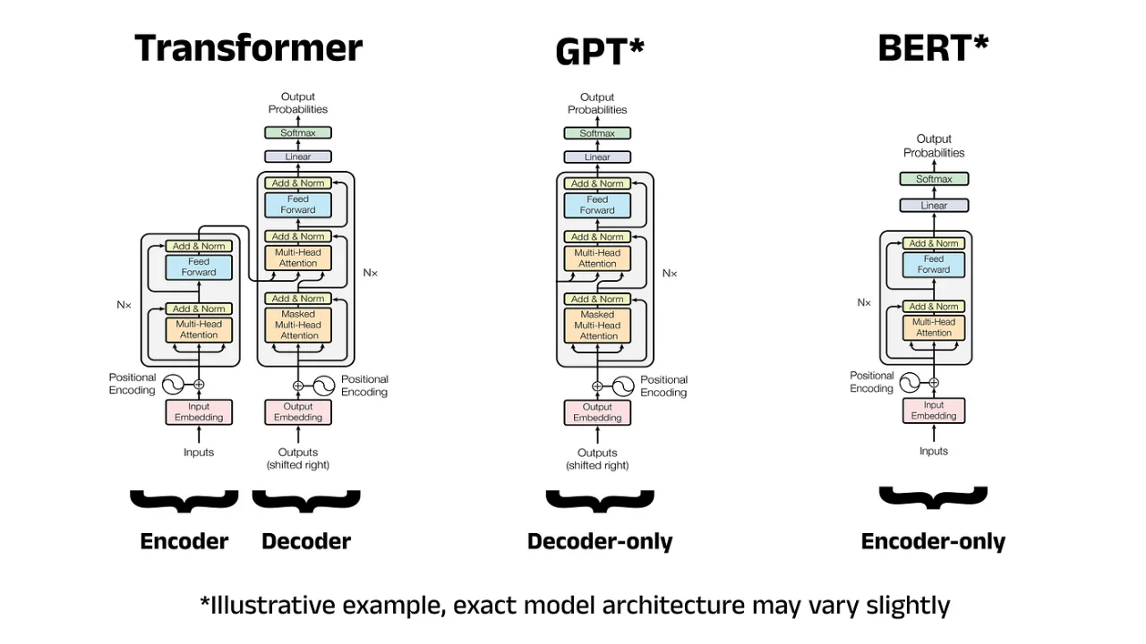
The paper “Attention is All You Need” debuted perhaps the single largest advancement in Natural Language Processing (NLP) in the last 10 years: the Transformer [1]. This architecture massively simplified the complex designs of language models at the time while achieving unparalleled results. State-of-the-art (SOTA) models, such as those in the GPT, Claude, and Llama families, owe their success to this design, at the heart of which is self-attention. In this deep dive, we will explore how this mechanism works and how it is used by transformers to create contextually rich embeddings that enable these models to perform so well.

Part 3 in the “LLMs from Scratch” series — a complete guide to understanding and building Large Language Models. If you are interested in learning more about how these models work I encourage you to read:

• Prelude: A Brief History of Large Language Models
• Part 1: Tokenization — A Complete Guide
• Part 2: Word Embeddings with word2vec from Scratch in Python
• Part 3: Self-Attention Explained with Code (Current article)
• Part 4: A Complete Guide to BERT with Code

1 — Overview of the Transformer Embedding Process

1.1 — Recap on Transformers

In the prelude article of this series, we briefly explored the history of the Transformer and its impact on NLP. To recap: the Transformer is a deep neural network architecture that is the foundation for almost all LLMs today. Derivative models are often called Transformer-based models or transformers for short, and so these terms will be used interchangeably here. Like all machine learning models, transformers work with numbers and linear algebra rather than processing human language directly. Because of this, they must convert textual inputs from users into numerical representations through several steps. Perhaps the most important of these steps is applying the self-attention mechanism, which is the focus of this article. The process of representing text with vectors is called embedding (or encoding), hence the numerical representations of the input text are known as transformer embeddings.

1.2 — The Issue with Static Embeddings

In Part 2 of this series, we explored static embeddings for language models using word2vec as an example. This embedding method predates transformers and suffers from one major drawback: the lack of contextual information. Words with multiple meanings (called polysemous words) are encoded with somewhat ambiguous representations since they lack the context needed for precise meaning. A classic example of a polysemous word is bank. Using a static embedding model, the word bank would be represented in vector space with some degree of similarity to words such as money and deposit and some degree of similarity to words such as river and nature. This is because the word will occur in many different contexts within the training data. This is the core problem with static embeddings: they do not change based on context — hence the term “static”.

1.3 — Fixing Static Embeddings

Transformers overcome the limitations of static embeddings by producing their own context-aware transformer embeddings. In this approach, fixed word embeddings are augmented with positional information (where the words occur in the input text) and contextual information (how the words are used). These two steps take place in distinct components in transformers, namely the positional encoder and the self-attention blocks, respectively. We will look at each of these in detail in the following sections. By incorporating this additional information, transformers can produce much more powerful vector representations of words based on their usage in the input sequence. Extending the vector representations beyond static embeddings is what enables Transformer-based models to handle polysemous words and gain a deeper understanding of language compared to previous models.

1.4 — Introducing Learned Embeddings

Much like the word2vec approach released four years prior, transformers store the initial vector representation for each token in the weights of a linear layer (a small neural network). In the word2vec model, these representations form the static embeddings, but in the Transformer context these are known as learned embeddings. In practice they are very similar, but using a different name emphasises that these representations are only a starting point for the transformer embeddings and not the final form.

The linear layer sits at the beginning of the Transformer architecture and contains only weights and no bias terms (bias = 0 for every neuron). The layer weights can be represented as a matrix of size V × d_model, where V is the vocabulary size (the number of unique words in the training data) and d_model is the number of embedding dimensions. In the previous article, we denoted d_model as N, in line with word2vec notation, but here we will use d_model which is more common in the Transformer context. The original Transformer was proposed with a d_model size of 512 dimensions, but in practice any reasonable value can be used.

A diagram showing the location of the linear layer in the Transformer architecture, which stores the learned embeddings. Image by author, adapted from the Transformer architecture diagram in the “Attention is All You Need” paper [1].

1.5 — Creating Learned Embeddings

A key difference between static and learned embeddings is the way in which they are trained. Static embeddings are trained in a separate neural network (using the Skip-Gram or Continuous Bag of Words architectures) using a word prediction task within a given window size. Once trained, the embeddings are then extracted and used with a range of different language models. Learned embeddings, however, are integral to the transformer you are using and are stored as weights in the first linear layer of the model. These weights, and consequently the learned embedding for each token in the vocabulary, are trained in the same backpropagation steps as the rest of the model parameters. Below is a summary of the training process for learned embeddings.

Step 1: Initialisation

Randomly initialise the weights for each neuron in the linear layer at the beginning of the model, and set the bias terms to 0. This layer is also called the embedding layer, since it is the linear layer that will store the learned embeddings. The weights can be represented as a matrix of size V × d_model, where the word embedding for each word in the vocabulary is stored along the rows. For example, the embedding for the first word in the vocabulary is stored in the first row, the second word is stored in the second row, and so on.

Step 2: Training

At each training step, the Transformer receives an input word and the aim is to predict the next word in the sequence — a task known as Next Token Prediction (NTP). Initially, these predictions will be very poor, and so every weight and bias term in the network will be updated to improve performance against the loss function, including the embeddings. After many training iterations, the learned embeddings should provide a strong vector representation for each word in the vocabulary.

Step 3: Extract the Learned Embeddings

When new input sequences are given to the model, the words are converted into tokens with an associated token ID, which corresponds to the position of the token in the tokenizer’s vocabulary. For example, the word cat may lie at position 349 in the tokenizer’s vocabulary and so will take the ID 349. Token IDs are used to create one-hot encoded vectors that extract the correct learned embeddings from the weights matrix (that is, V-dimensional vectors where every element is 0 except for the element at the token ID position, which is 1).

Note: "PyTorch is a very popular deep learning library in Python that powers some of the most well-known machine learning packages, such as the HuggingFace Transformers library [2]. If you are familiar with PyTorch, you may have encountered the nn.Embedding class, which is often used to form the first layer of transformer networks (the nn denotes that the class belongs to the neural network package). This class returns a regular linear layer that is initialised with the identity function as the activation function and with no bias term. The weights are randomly initialised since they are parameters to be learned by the model during training. This essentially carries out the steps described above in one simple line of code. Remember, the nn.Embeddings layer does not provide pre-trained word embeddings out-of-the-box, but rather initialises a blank canvas of embeddings before training. This is to allow the transformer to learn its own embeddings during the training phase."

1.6 — Transformer Embedding Process

Once the learned embeddings have been trained, the weights in the embedding layer never change. That is, the learned embedding for each word (or more specifically, token) always provides the same starting point for a word’s vector representation. From here, the positional and contextual information will be added to produce a unique representation of the word that is reflective of its usage in the input sequence.

Transformer embeddings are created in a four-step process, which is demonstrated below using the example prompt: Write a poem about a man fishing on a river bank. Note that the first two steps are the same as the word2vec approach we saw before. Steps 3 and 4 are the further processing that add contextual information to the embeddings.

Step 1) Tokenization:

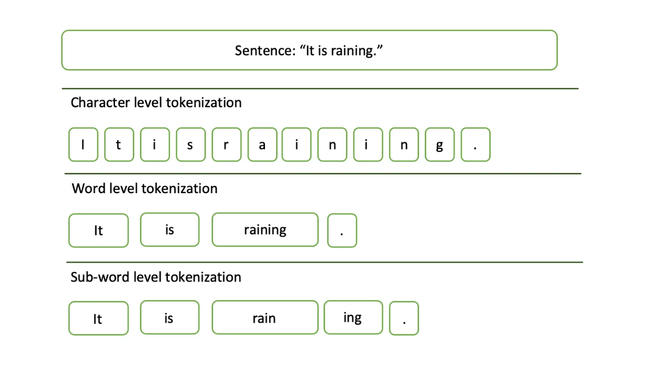
Tokenization is the process of dividing a longer input sequence into individual words (and parts of words) called tokens. In this case, the sentence will be broken down into:
write, a, poem, about, a, man, fishing, on, a, river, bank

Next, the tokens are associated with their token IDs, which are integer values corresponding to the position of the token in the tokenizer’s vocabulary (see Part 1 of this series for an in-depth look at the tokenization process).

Step 2) Map the Tokens to Learned Embeddings:

Once the input sequence has been converted into a set of token IDs, the tokens are then mapped to their learned embedding vector representations, which were acquired during the transformer’s training. These learned embeddings have the “lookup table” behaviour as we saw in the word2vec example in Part 2 of this series. The mapping takes place by multiplying a one-hot encoded vector created from the token ID with the weights matrix, just as in the word2vec approach. The learned embeddings are denoted V in the image below.

Step 3) Add Positional Information with Positional Encoding:

Positional Encoding is then used to add positional information to the word embeddings. Whereas Recurrent Neural Networks (RNNs) process text sequentially (one word at a time), transformers process all words in parallel. This removes any implicit information about the position of each word in the sentence. For example, the sentences the cat ate the mouse and the mouse ate the cat use the same words but have very different meanings. To preserve the word order, positional encoding vectors are generated and added to the learned embedding for each word. In the image below, the positional encoding vectors are denoted P, and the sums of the learned embeddings and positional encodings are denoted X.

Step 4) Modify the Embeddings using Self-Attention:

The final step is to add contextual information using the self-attention mechanism. This determines which words give context to other words in the input sequence. In the image below, the transformer embeddings are denoted y.

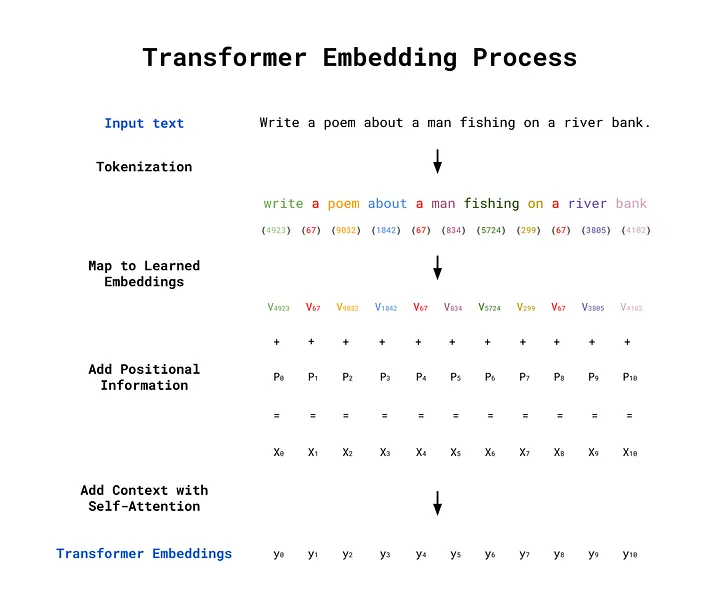
An overview of the transformer embedding process from input text through to transformer embeddings. Image by author.

2 — Positional Encoding

2.1 — The Need for Positional Encoding

Before the self-attention mechanism is applied, positional encoding is used to add information about the order of tokens to the learned embeddings. This compensates for the loss of positional information caused by the parallel processing used by transformers described earlier. There are many feasible approaches for injecting this information, but all methods must adhere to a set of constraints. The functions used to generate positional information must produce values that are:

• Bounded — values should not explode in the positive or negative direction but be constrained (e.g. between 0 and 1, -1 and 1, etc)
• Periodic — the function should produce a repeating pattern that the model can learn to recognise and discern position from
• Predictable — positional information should be generated in such a way that the model can understand the position of words in sequence lengths it was not trained on. For example, even if the model has not seen a sequence length of exactly 412 tokens in its training, the transformer should be able to understand the position of each of the embeddings in the sequence.

These constraints ensure that the positional encoder produces positional information that allows words to attend to (gain context from) any other important word, regardless of their relative positions in the sequence. In theory, with a sufficiently powerful computer, words should be able to gain context from every relevant word in an infinitely long input sequence. The length of a sequence from which a model can derive context is called the context length. In chatbots like ChatGPT, the context includes the current prompt as well as all previous prompts and responses in the conversation (within the context length limit). This limit is typically in the range of a few thousand tokens, with GPT-3 supporting up to 4096 tokens and GPT-4 enterprise edition capping at around 128,000 tokens [3].

2.2 — Positional Encoding in “Attention is All You Need”

The original transformer model was proposed with the following positional encoding functions:

An image of the equations for positional encoding, as proposed in the paper “Attention is All You Need” [1]. Image by author.

where:

• pos is the position of the word in the input, where pos = 0 corresponds to the first word in the sequence
• i is the index of each embedding dimension, ranging from i=0 (for the first embedding dimension) up to d_model
• d_model is the number of embedding dimensions for each learned embedding vector (and therefore each positional encoding vector). This was previously denoted N in the article on word2vec.

The two proposed functions take arguments of 2i and 2i+1, which in practice means that the sine function generates positional information for the even-numbered dimensions of each word vector (i is even), and the cosine function does so for the odd-numbered dimensions (i is odd). According to the authors of the transformer:

“The positional encoding corresponds to a sinusoid. The wavelengths form a geometric progression from 2π to 10000·2π. We chose this function because we hypothesised it would allow the model to easily learn to attend by relative positions, since for any fixed offset k, PE_pos+k can be represented as a linear function of PE_pos”.

The value of the constant in the denominator being 10_000 was found to be suitable after some experimentation, but is a somewhat arbitrary choice by the authors.

2.3 — Other Positional Encoding Approaches

The positional encodings shown above are considered fixed because they are generated by a known function with deterministic (predictable) outputs. This represents the most simple form of positional encoding. It is also possible to use learned positional encodings by randomly initialising some positional encodings and training them with backpropagation. Derivatives of the BERT architecture are examples of models that take this learned encoding approach. More recently, the Rotary Positional Encoding (RoPE) method has gained popularity, finding use in models such as Llama 2 and PaLM, among other positional encoding methods.

2.4 — Implementing a Positional Encoder in Python

Creating a positional encoder class in Python is fairly straightforward. We can start by defining a function that accepts the number of embedding dimensions (d_model), the maximum length of the input sequence (max_length), and the number of decimal places to round each value in the vectors to (rounding). Note that transformers define a maximum input sequence length, and any sequence that has fewer tokens than this limit is appended with padding tokens until the limit is reached. To account for this behaviour in our positional encoder, we accept a max_length argument. In practice, this limit is typically thousands of characters long.

We can also exploit a mathematical trick to save computation. Instead of calculating the denominator for both PE_{pos, 2i} and PE_{pos, 2i}, we can note that the denominator is identical for consecutive pairs of i. For example, the denominators for i=0 and i=1 are the same, as are the denominators for i=2 and i=3. Hence, we can perform the calculations to determine the denominators once for the even values of i and reuse them for the odd values of i.

import numpy as np

class PositionalEncoder():
    """ An implementation of positional encoding.

    Attributes:
        d_model (int): The number of embedding dimensions in the learned
            embeddings. This is used to determine the length of the positional
            encoding vectors, which make up the rows of the positional encoding
            matrix.
        max_length (int): The maximum sequence length in the transformer. This
            is used to determine the size of the positional encoding matrix.
        rounding (int): The number of decimal places to round each of the
            values to in the output positional encoding matrix.
    """

    def __init__(self, d_model, max_length, rounding):
        self.d_model = d_model
        self.max_length = max_length
        self.rounding = rounding

    def generate_positional_encoding(self):
        """ Generate positional information to add to inputs for encoding.

        The positional information is generated using the number of embedding
        dimensions (d_model), the maximum length of the sequence (max_length),
        and the number of decimal places to round to (rounding). The output
        matrix generated is of size (max_length X embedding_dim), where each
        row is the positional information to be added to the learned
        embeddings, and each column is an embedding dimension.
        """

        position = np.arange(0, self.max_length).reshape(self.max_length, 1)
        even_i = np.arange(0, self.d_model, 2)
        denominator = 10_000**(even_i / self.d_model)

        even_encoded = np.round(np.sin(position / denominator), self.rounding)
        odd_encoded = np.round(np.cos(position / denominator), self.rounding)

        # Interleave the even and odd encodings
        positional_encoding = np.stack((even_encoded, odd_encoded),2)\
        .reshape(even_encoded.shape[0],-1)

        # If self.d_model is odd remove the extra column generated
        if self.d_model % 2 == 1:
            positional_encoding = np.delete(positional_encoding, -1, axis=1)

        return positional_encoding

    def encode(self, input):
        """ Encode the input by adding positional information.

        Args:
            input (np.array): A two-dimensional array of embeddings. The array
                should be of size (self.max_length x self.d_model).

        Returns:
            output (np.array): A two-dimensional array of embeddings plus the
                positional information. The array has size (self.max_length x
                self.d_model).
        """
        positional_encoding = self.generate_positional_encoding()
        output = input + positional_encoding

        return output

MAX_LENGTH = 5
EMBEDDING_DIM = 3
ROUNDING = 2

# Instantiate the encoder
PE = PositionalEncoder(d_model=EMBEDDING_DIM,
                       max_length=MAX_LENGTH,
                       rounding=ROUNDING)

# Create an input matrix of word embeddings without positional encoding
input = np.round(np.random.rand(MAX_LENGTH, EMBEDDING_DIM), ROUNDING)

# Create an output matrix of word embeddings by adding positional encoding
output = PE.encode(input)

# Print the results
print(f'Embeddings without positional encoding:\n\n{input}\n')
print(f'Positional encoding:\n\n{output-input}\n')
print(f'Embeddings with positional encoding:\n\n{output}')

Embeddings without positional encoding:

[[0.12 0.94 0.9 ]
 [0.14 0.65 0.22]
 [0.29 0.58 0.31]
 [0.69 0.37 0.62]
 [0.25 0.61 0.65]]

Positional encoding:

[[ 0.    1.    0.  ]
 [ 0.84  0.54  0.  ]
 [ 0.91 -0.42  0.  ]
 [ 0.14 -0.99  0.01]
 [-0.76 -0.65  0.01]]

Embeddings with positional encoding:

[[ 0.12  1.94  0.9 ]
 [ 0.98  1.19  0.22]
 [ 1.2   0.16  0.31]
 [ 0.83 -0.62  0.63]
 [-0.51 -0.04  0.66]]

2.5 — Visualising the Positional Encoding Matrix

Recall that the positional information generated must be bounded, periodic, and predictable. The outputs of the sinusoidal functions presented earlier can be collected into a matrix, which can then be easily combined with the learned embeddings using element-wise addition. Plotting this matrix gives a nice visualisation of the desired properties. In the plot below, curving bands of negative values (blue) emanate from the left edge of the matrix. These bands form a pattern that the transformer can easily learn to predict.

import matplotlib.pyplot as plt

# Instantiate a PositionalEncoder class
d_model = 400
max_length = 100
rounding = 4

PE = PositionalEncoder(d_model=d_model,
                       max_length=max_length,
                       rounding=rounding)

# Generate positional encodings
input = np.round(np.random.rand(max_length, d_model), 4)
positional_encoding = PE.generate_positional_encoding()

# Plot positional encodings
cax = plt.matshow(positional_encoding, cmap='coolwarm')
plt.title(f'Positional Encoding Matrix ({d_model=}, {max_length=})')
plt.ylabel('Position of the Embedding\nin the Sequence, pos')
plt.xlabel('Embedding Dimension, i')
plt.gcf().colorbar(cax)
plt.gca().xaxis.set_ticks_position('bottom')

A visualisation of the positional encoding matrix for a model with 400 embedding dimensions (d_model = 400), and a maximum sequence length of 100 (max_length = 100). Image by author.

3 — The Self-Attention Mechanism

3.1 — Overview of Attention Mechanisms

Now that we have covered an overview of transformer embeddings and the positional encoding step, we can turn our focus to the self-attention mechanism itself. In short, self-attention modifies the vector representation of words to capture the context of their usage in an input sequence. The “self” in self-attention refers to the fact that the mechanism uses the surrounding words within a single sequence to provide context. As such, self-attention requires all words to be processed in parallel. This is actually one of the main benefits of transformers (especially compared to RNNs) since the models can leverage parallel processing for a significant performance boost. In recent times, there has been some rethinking around this approach, and in the future we may see this core mechanism being replaced [4].

Another form of attention used in transformers is cross-attention. Unlike self-attention, which operates within a single sequence, cross-attention compares each word in an output sequence to each word in an input sequence, crossing between the two embedding matrices. Note the difference here compared to self-attention, which focuses entirely within a single sequence.

3.2 — Visualising How Self-Attention Contextualises Embeddings

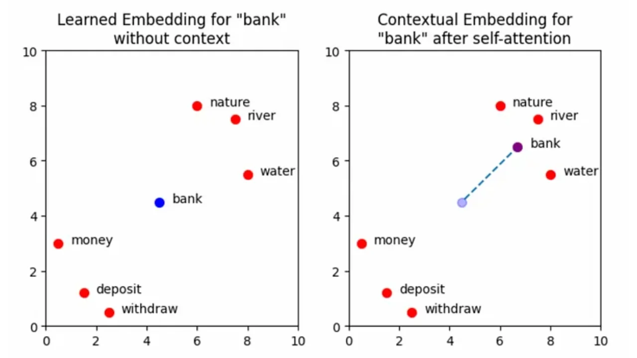
The plots below show a simplified set of learned embedding vectors in two dimensions. Words associated with nature and rivers are concentrated in the top right quadrant of the graph, while words associated with money are concentrated in the bottom left. The vector representing the word bank is positioned between the two clusters due to its polysemic nature. The objective of self-attention is to move the learned embedding vectors to regions of vector space that more accurately capture their meaning within the context of the input sequence. In the example input Write a poem about a man fishing on a river bank, the aim is to move the vector for bank in such a way that captures more of the meaning of nature and rivers, and less of the meaning of money and deposits.

Note: More accurately, the goal of self-attention here is to update the vector for every word in the input, so that all embeddings better represent the context in which they were used. There is nothing special about the word bank here that transformers have some special knowledge of — self-attention is applied across all the words. We will look more at this shortly, but for now, considering solely how bank is affected by self-attention gives a good intuition for what is happening in the attention block. For the purpose of this visualisation, the positional encoding information has not been explicitly shown. The effect of this will be minimal, but note that the self-attention mechanism will technically operate on the sum of the learned embedding plus the positional information and not solely the learned embedding itself.

import matplotlib.pyplot as plt

# Create word embeddings
xs = [0.5, 1.5, 2.5, 6.0, 7.5, 8.0]
ys = [3.0, 1.2, 0.5, 8.0, 7.5, 5.5]
words = ['money', 'deposit', 'withdraw', 'nature', 'river', 'water']
bank = [[4.5, 4.5], [6.7, 6.5]]

# Create figure
fig, ax = plt.subplots(ncols=2, figsize=(8,4))

# Add titles
ax[0].set_title('Learned Embedding for "bank"\nwithout context')
ax[1].set_title('Contextual Embedding for\n"bank" after self-attention')

# Add trace on plot 2 to show the movement of "bank"
ax[1].scatter(bank[0][0], bank[0][1], c='blue', s=50, alpha=0.3)
ax[1].plot([bank[0][0]+0.1, bank[1][0]],
           [bank[0][1]+0.1, bank[1][1]],
           linestyle='dashed',
           zorder=-1)

for i in range(2):
    ax[i].set_xlim(0,10)
    ax[i].set_ylim(0,10)

    # Plot word embeddings
    for (x, y, word) in list(zip(xs, ys, words)):
        ax[i].scatter(x, y, c='red', s=50)
        ax[i].text(x+0.5, y, word)

    # Plot "bank" vector
    x = bank[i][0]
    y = bank[i][1]

    color = 'blue' if i == 0 else 'purple'

    ax[i].text(x+0.5, y, 'bank')
    ax[i].scatter(x, y, c=color, s=50)

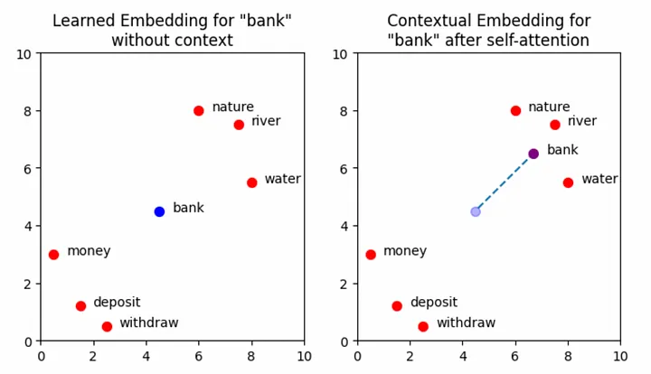
A visualisation of the vector representation for the word “bank” moving through the embedding space following the addition of contextual information. Image by author

3.3 — The Self-Attention Algorithm

In the section above, we stated that the goal of self-attention is to move the embedding for each token to a region of vector space that better represents the context of its use in the input sequence. What we didn’t discuss is how this is done. Here we will show a step-by-step example of how the self-attention mechanism modifies the embedding for bank, by adding context from the surrounding tokens.

A simplified overview of a self-attention block (with the key, query, and value matrices excluded). Image by author.

Step 1) Calculate the Similarity Between Words using the Dot Product:

The context of a token is given by the surrounding tokens in the sentence. Therefore, we can use the embeddings of all the tokens in the input sequence to update the embedding for any word, such as bank. Ideally, words that provide significant context (such as river) will heavily influence the embedding, while words that provide less context (such as a) will have minimal effect.

The degree of context one word contributes to another is measured by a similarity score. Tokens with similar learned embeddings are likely to provide more context than those with dissimilar embeddings. The similarity scores are calculated by taking the dot product of the current embedding for one token (its learned embedding plus positional information) with the current embeddings of every other token in the sequence. For clarity, the current embeddings have been termed self-attention inputs in this article and are denoted x.

There are several options for measuring the similarity between two vectors, which can be broadly categorised into: distance-based and angle-based metrics. Distance-based metrics characterise the similarity of vectors using the straight-line distance between them. This calculation is relatively simple and can be thought of as applying Pythagoras’s theorem in d_model-dimensional space. While intuitive, this approach is computationally expensive.

For angle-based similarity metrics, the two main candidates are: cosine similarity and dot-product similarity. Both of these characterise similarity using the cosine of the angle between the two vectors, θ. For orthogonal vectors (vectors that are at right angles to each other) cos(θ) = 0, which represents no similarity. For parallel vectors, cos(θ) = 1, which represents that the vectors are identical. Solely using the angle between vectors, as is the case with cosine similarity, is not ideal for two reasons. The first is that the magnitude of the vectors is not considered, so distant vectors that happen to be aligned will produce inflated similarity scores. The second is that cosine similarity requires first computing the dot product and then dividing by the product of the vectors’ magnitudes — making cosine similarity a computationally expensive metric. Therefore, the dot product is used to determine similarity. The dot product formula is given below for two vectors x_1 and x_2.

The dot product formula for two vectors x_1 and x_2. Image by author.

The diagram below shows the dot product between the self-attention input vector for bank, x_bank, and the matrix of vector representations for every token in the input sequence, X^T. We can also write x_bank as x_11 to reflect its position in the input sequence. The matrix X stores the self-attention inputs for every token in the input sequence as rows. The number of columns in this matrix is given by L_max, the maximum sequence length of the model. In this example, we will assume that the maximum sequence length is equal to the number of words in the input prompt, removing the need for any padding tokens (see Part 4 in this series for more about padding). To compute the dot product directly, we can transpose X and calculate the vector of similarity scores, S_bank using S_bank = x_bank ⋅ X^T. The individual elements of S_bank represent the similarity scores between bank and each token in the input sequence.

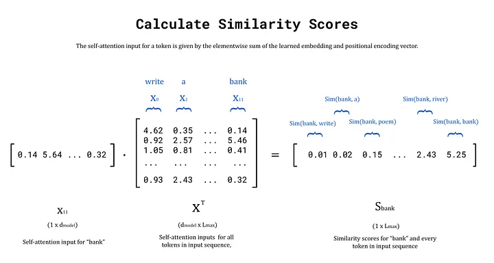
An example calculation of the similarity scores for X_11 with every self-attention input (the sum of the learned embedding and positional information for each token in the input sequence). Image by author

Step 2) Scale the Similarity Scores:

The dot product approach lacks any form of normalisation (unlike cosine similarity), which can cause the similarity scores to become very large. This can pose computational challenges, so normalisation of some form becomes necessary. The most common method is to divide each score by √d_model, resulting in scaled dot-product attention. Scaled dot-product attention is not restricted to self-attention and is also used for cross-attention in transformers.

Step 3) Calculate the Attention Weights using the Softmax Function:

The output of the previous step is the vector S_bank, which contains the similarity scores between bank and every token in the input sequence. These similarity scores are used as weights to construct a transformer embedding for bank from the weighted sum of embeddings for each surrounding token in the prompt. The weights, known as attention weights, are calculated by passing S_bank into the softmax function. The outputs are stored in a vector denoted W_bank. To see more about the softmax function, refer to the previous article on word2vec.

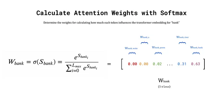
An example calculation of the attention weights for “bank” based on the similarity with every self-attention input. Image by author

Step 4) Calculate the Transformer Embedding

Finally, the transformer embedding for bank is obtained by taking the weighted sum of write, a, prompt, …, bank. Of course, bank will have the highest similarity score with itself (and therefore the largest attention weight), so the output embedding after this process will remain similar to before. This behaviour is ideal since the initial embedding already occupies a region of vector space that encodes some meaning for bank. The goal is to nudge the embedding towards the words that provide more context. The weights for words that provide little context, such as a and man, are very small. Hence, their influence on the output embedding will be minimal. Words that provide significant context, such as river and fishing, will have higher weights, and therefore pull the output embedding closer to their regions of vector space. The end result is a new embedding, y_bank, that reflects the context of the entire input sequence.

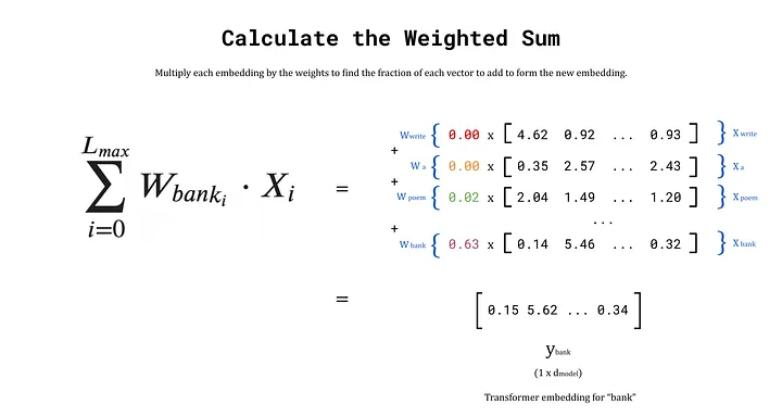
An example calculation for the new embedding of “bank” by taking a weighted sum of the other embeddings for each token in the sequence. Image by author

3.4 — Expanding Self-Attention using Matrices

Above, we walked through the steps to calculate the transformer embedding for the singular word bank. The input consisted of the learned embedding vector for bank plus its positional information, which we denoted x_11 or x_bank. The key point here, is that we considered only one vector as the input. If we instead pass in the matrix X (with dimensions L_max × d_model) to the self-attention block, we can calculate the transformer embedding for every token in the input prompt simultaneously. The output matrix, Y, contains the transformer embedding for every token along the rows of the matrix. This approach is what enables transformers to quickly process text.

A black box diagram of a self-attention block. The matrix of word vectors is represented by X for the input sequence, and Y for the output sequence. Image by author

3.5 — The Query, Key, and Value Matrices

The above description gives an overview of the core functionality of the self-attention block, but there is one more piece of the puzzle. The simple weighted sum above does not include any trainable parameters, but we can introduce some to the process. Without trainable parameters, the performance of the model may still be good, but by allowing the model to learn more intricate patterns and hidden features from the training data, we observe much stronger model performance.

The self-attention inputs are used three times to calculate the new embeddings, these include the x_bank vector, the X^T matrix in the dot product step, and the X^T matrix in the weighted sum step. These three sites are the perfect candidates to introduce some weights, which are added in the form of matrices (shown in red). When pre-multiplied by their respective inputs (shown in blue), these form the key, query, and value matrices, K, Q, and V (shown in purple). The number of columns in these weight matrices is an architectural choice by the user. Choosing a value for d_q, d_k, and d_v that is less than d_model will result in dimensionality reduction, which can improve model speed. Ultimately, these values are hyperparameters that can be changed based on the specific implementation of the model and the use-case, and are often all set equal to d_model if unsure [5].

A diagram of a complete self-attention block including the key, query, and value matrices. Image by author

3.6 — The Database Analogy

The names for these matrices come from an analogy with databases, which is explained briefly below.

Query:

• A query in a database is what you are looking for when performing a search. For example, “show me all the albums in the database that have sold more than 1,000,000 records”. In the self-attention block, we are essentially asking the same question, but phrased as “show me the transformer embedding for this vector (e.g. x_bank)”.

Key:

• The keys in the database are the attributes or columns that are being searched against. In the example given earlier, you can think of this as the “Albums Sold” column, which stores the information we are interested in. In self-attention, we are interested in the embeddings for every word in the input prompt, so we can compute a set of attention weights. Therefore, the key matrix is a collection of all the input embeddings.

Value:

• The values correspond to the actual data in the database, that is, the actual sale figures in our example (e.g. 2,300,000 copies). For self-attention, this is exactly the same as the input for the key matrix: a collection of all the input embeddings. Hence, the key and value matrices both take in the matrix X as the input.

3.7 — A Note on Multi-Head Attention

Distributing Computation Across Multiple Heads:

The “Attention is All You Need” paper expands self-attention into multi-head attention, which gives even richer representations of the input sequences. This method involves repeating the calculation of attention weights using different key, query, and value matrices which are learned independently within each head. A head is a section of the attention block dedicated to processing a fraction of the input embedding dimensions. For example, an input, x, with 512 dimensions will be divided by the number of heads, h, to create h chunks of size d_k (where d_k = d_model / h). For a model with 8 heads (h=8), each head will receive 64 dimensions of x (d_k = 64). Each chunk is processed using the self-attention mechanism in its respective head, and at the end the outputs from all heads are combined using a linear layer to produce a single output with the original 512 dimensions.

The Benefits of Using Multiple Heads:

The core idea is to allow each head to learn different types of relationships between words in the input sequence, and to combine them to create deep text representations. For example, some heads might learn to capture long-term dependencies (relationships between words that are distant in the text), while others might focus on short-term dependencies (words that are close in text).

Building Intuition for Multi-Head Attention:

To build some intuition for the usefulness of multiple attention heads, consider words in a sentence that require a lot of context. For example, in the sentence I ate some of Bob’s chocolate cake, the word ate should attend to I, Bob’s and cake to gain full context. This is a rather simple example, but if you extend this concept to complex sequences spanning thousands of words, hopefully it seems reasonable that distributing the computational load across separate attention mechanisms will be beneficial.

An example of attention heads capturing different word dependencies in an input sequence. Image by author

Summary of Multi-Head Attention:

To summarise, multi-head attention involves repeating the self-attention mechanism h times and combining the results to distil the information into rich transformer embeddings. While this step is not strictly necessary, it has been found to produce more impressive results, and so is standard in transformer-based models.

A diagram of a multi-head attention block showing h attention heads acting on an example input. Image by author

4 — Transformer Embeddings in Python

4.1 — Extracting Learned Embeddings and Transformer Embeddings from Transformer Models

Python has many options for working with transformer models, but none are perhaps as well-known as Hugging Face. Hugging Face provides a centralised resource hub for NLP researchers and developers alike, including tools such as:

• transformers: The library at the core of Hugging Face, which provides an interface for using, training, and fine-tuning pre-trained transformer models.
• tokenizers: A library for working with tokenizers for many kinds of transformers, either using pre-built tokenizer models or constructing brand new ones from scratch.
• datasets: A collection of datasets to train models on a variety of tasks, not just restricted to NLP.
• Model Hub: A large repository of cutting-edge models from published papers, community-developed models, and everything in between. These are made freely available and can be easily imported into Python via the transformers API.

The code cell below shows how the transformers library can be used to load a transformer-based model into Python, and how to extract both the learned embeddings for words (without context) and the transformer embeddings (with context). The remainder of this article will break down the steps shown in this cell and describe additional functionalities available when working with embeddings.

import torch
from transformers import AutoModel, AutoTokenizer

def extract_le(sequence, tokenizer, model):
    """ Extract the learned embedding for each token in an input sequence.

    Tokenize an input sequence (string) to produce a tensor of token IDs.
    Return a tensor containing the learned embedding for each token in the
    input sequence.

    Args:
        sequence (str): The input sentence(s) to tokenize and extract
            embeddings from.
        tokenizer: The tokenizer used to produce tokens.
        model: The model to extract learned embeddings from.

    Returns:
        learned_embeddings (torch.tensor): A tensor containing tensors of
            learned embeddings for each token in the input sequence.
    """
    token_dict = tokenizer(sequence, return_tensors='pt')
    token_ids = token_dict['input_ids']
    learned_embeddings = model.embeddings.word_embeddings(token_ids)[0]

    # Additional processing for display purposes
    learned_embeddings = learned_embeddings.tolist()
    learned_embeddings = [[round(i,2) for i in le] \
                          for le in learned_embeddings]

    return learned_embeddings

def extract_te(sequence, tokenizer, model):
    """ Extract the tranformer embedding for each token in an input sequence.

    Tokenize an input sequence (string) to produce a tensor of token IDs.
    Return a tensor containing the transformer embedding for each token in the
    input sequence.

    Args:
        sequence (str): The input sentence(s) to tokenize and extract
            embeddings from.
        tokenizer: The tokenizer used to produce tokens.
        model: The model to extract learned embeddings from.

    Returns:
        transformer_embeddings (torch.tensor): A tensor containing tensors of
            transformer embeddings for each token in the input sequence.
    """
    token_dict = tokenizer(sequence, return_tensors='pt')

    with torch.no_grad():
        base_model_output = model(**token_dict)

    transformer_embeddings = base_model_output.last_hidden_state[0]

    # Additional processing for display purposes
    transformer_embeddings = transformer_embeddings.tolist()
    transformer_embeddings = [[round(i,2) for i in te] \
                              for te in transformer_embeddings]

    return transformer_embeddings

# Instantiate DistilBERT tokenizer and model
tokenizer = AutoTokenizer.from_pretrained('distilbert-base-uncased')
model = AutoModel.from_pretrained('distilbert-base-uncased')

# Extract the learned embedding for bank from DistilBERT
le_bank = extract_le('bank', tokenizer, model)[1]

# Write sentences containing "bank" in two different contexts
s1 = 'Write a poem about a man fishing on a river bank.'
s2 = 'Write a poem about a man withdrawing money from a bank.'

# Extract the transformer embedding for bank from DistilBERT in each sentence
s1_te_bank = extract_te(s1, tokenizer, model)[11]
s2_te_bank = extract_te(s2, tokenizer, model)[11]

# Print the results
print('------------------- Embedding vectors for "bank" -------------------\n')
print(f'Learned embedding:                  {le_bank[:5]}')
print(f'Transformer embedding (sentence 1): {s1_te_bank[:5]}')
print(f'Transformer embedding (sentence 2): {s2_te_bank[:5]}')

------------------- Embedding vectors for "bank" -------------------

Learned embedding:                  [-0.03, -0.06, -0.09, -0.07, -0.03]
Transformer embedding (sentence 1): [0.15, -0.16, -0.17, -0.08, 0.44]
Transformer embedding (sentence 2): [0.27, -0.23, -0.23, -0.21, 0.79]

4.2 — Import the Transformers Library

The first step to produce transformer embeddings is to choose a model from the Hugging Face transformers library. In this article, we will not use the model for inference but solely to examine the embeddings it produces. This is not a standard use-case, and so we will have to do some extra digging in order to access the embeddings. Since the transformers library is written in PyTorch (referred to as torch in the code), we can import torch to extract data from the inner workings of the models.

4.3 — Choose a Model

For this example, we will use DistilBERT, a smaller version of Google’s BERT model which was released by Hugging Face themselves in October 2019 [6]. According to the Hugging Face documentation [7]:

DistilBERT is a small, fast, cheap and light Transformer model trained by distilling BERT base. It has 40% less parameters than bert-base-uncased, runs 60% faster while preserving over 95% of BERT’s performances as measured on the GLUE language understanding benchmark.

We can import DistilBERT and its corresponding tokenizer into Python either directly from the transformers library or using the AutoModel and AutoTokenizer classes. There is very little difference between the two, although AutoModel and AutoTokenizer are often preferred since the model name can be parameterised and stored in a string, which makes it simpler to change the model being used.

import torch
from transformers import DistilBertTokenizerFast, DistilBertModel

# Instantiate DistilBERT tokenizer and model
tokenizer = DistilBertTokenizerFast.from_pretrained('distilbert-base-uncased')
model = DistilBertModel.from_pretrained('distilbert-base-uncased')

import torch
from transformers import AutoModel, AutoTokenizer

# Instantiate DistilBERT tokenizer and model
tokenizer = AutoTokenizer.from_pretrained('distilbert-base-uncased')
model = AutoModel.from_pretrained('distilbert-base-uncased')

After importing DistilBERT and its corresponding tokenizer, we can call the from_pretrained method for each to load in the specific version of the DistilBERT model and tokenizer we want to use. In this case, we have chosen distilbert-base-uncased, where base refers to the size of the model, and uncased indicates that the model was trained on uncased text (all text is converted to lowercase).

4.4 — Create Some Example Sentences

Next, we can create some sentences to give the model some words to embed. The two sentences, s1 and s2, both contain the word bank but in different contexts. The goal here is to show that the word bank will begin with the same learned embedding in both sentences, then be modified by DistilBERT using self-attention to produce a unique, contextualised embedding for each input sequence.

# Create example sentences to produce embeddings for
s1 = 'Write a poem about a man fishing on a river bank.'
s2 = 'Write a poem about a man withdrawing money from a bank.'

4.5 — Tokenize an Input Sequence

The tokenizer class can be used to tokenize an input sequence (as shown below) and convert a string into a list of token IDs. Optionally, we can also pass a return_tensors argument to format the token IDs as a PyTorch tensor (return_tensors=pt) or as TensorFlow constants (return_tensors=tf). Leaving this argument empty will return the token IDs in a Python list. The return value is a dictionary that contains input_ids: the list-like object containing token IDs, and attention_mask which we will ignore for now.

Note: BERT-based models include a [CLS] token at the beginning of each sequence, and a [SEP] token to distinguish between two bodies of text in the input. These are present due to the tasks that BERT was originally trained on and can largely be ignored here. For a discussion on BERT special tokens, model sizes, cased vs uncased, and the attention mask, see Part 4 of this series.

token_dict = tokenizer(s1, return_tensors='pt')
token_ids = token_dict['input_ids'][0]

4.6 — Extract the Learned Embeddings from a Model

Each transformer model provides access to its learned embeddings via the embeddings.word_embeddings method. This method accepts a token ID or collection of token IDs and returns the learned embedding(s) as a PyTorch tensor.

learned_embeddings = model.embeddings.word_embeddings(token_ids)
learned_embeddings

tensor([[ 0.0390, -0.0123, -0.0208,  ...,  0.0607,  0.0230,  0.0238],
        [-0.0300, -0.0070, -0.0247,  ...,  0.0203, -0.0566, -0.0264],
        [ 0.0062,  0.0100,  0.0071,  ..., -0.0043, -0.0132,  0.0166],
        ...,
        [-0.0261, -0.0571, -0.0934,  ..., -0.0351, -0.0396, -0.0389],
        [-0.0244, -0.0138, -0.0078,  ...,  0.0069,  0.0057, -0.0016],
        [-0.0199, -0.0095, -0.0099,  ..., -0.0235,  0.0071, -0.0071]],
       grad_fn=<EmbeddingBackward0>)

4.7 — Extract the Transformer Embeddings from a Model

Converting a context-lacking learned embedding into a context-aware transformer embedding requires a forward pass of the model. Since we are not updating the weights of the model here (i.e. training the model), we can use the torch.no_grad() context manager to save on memory. This allows us to pass the tokens directly into the model and compute the transformer embeddings without any unnecessary calculations. Once the tokens have been passed into the model, a BaseModelOutput is returned, which contains various information about the forward pass. The only data that is of interest here is the activations in the last hidden state, which form the transformer embeddings. These can be accessed using the last_hidden_state attribute, as shown below, which concludes the explanation for the code cell shown at the top of this section.

with torch.no_grad():
    base_model_output = model(**token_dict)

transformer_embeddings = base_model_output.last_hidden_state
transformer_embeddings

tensor([[[-0.0957, -0.2030, -0.5024,  ...,  0.0490,  0.3114,  0.1348],
         [ 0.4535,  0.5324, -0.2670,  ...,  0.0583,  0.2880, -0.4577],
         [-0.1893,  0.1717, -0.4159,  ..., -0.2230, -0.2225,  0.0207],
         ...,
         [ 0.1536, -0.1616, -0.1735,  ..., -0.3608, -0.3879, -0.1812],
         [-0.0182, -0.4264, -0.6702,  ...,  0.3213,  0.5881, -0.5163],
         [ 0.7911,  0.2633, -0.4892,  ..., -0.2303, -0.6364, -0.3311]]])

4.8 — Convert Token IDs to Tokens

It is possible to convert token IDs back into textual tokens, which shows exactly how the tokenizer divided the input sequence. This is useful when longer or rarer words are divided into multiple subwords when using subword tokenizers such as WordPiece (e.g. in BERT-based models) or Byte-Pair Encoding (e.g. in the GPT family of models).

tokens = tokenizer.convert_ids_to_tokens(token_ids)
tokens

['[CLS]', 'write', 'a', 'poem', 'about', 'a', 'man', 'fishing', 'on', 'a',
 'river', 'bank', '.', '[SEP]']

5 — Conclusion

The self-attention mechanism generates rich, context-aware transformer embeddings for text by processing each token in an input sequence simultaneously. These embeddings build on the foundations of static word embeddings (such as word2vec) and enable more capable language models such as BERT and GPT. Further work in this field will continue to improve the capabilities of LLMs and NLP as a whole.

6 — Further Reading

[1] A. Vaswani, N. Shazeer, N. Parmar, J. Uszkoreit, L. Jones, A. N. Gomez, Ł. Kaiser, and I. Polosukhin, Attention is All You Need (2017), Advances in Neural Information Processing Systems 30 (NIPS 2017)
[2] Hugging Face, Transformers (2024), HuggingFace.co
[3] OpenAI, ChatGPT Pricing (2024), OpenAI.com
[4] A. Gu and T. Dao, Mamba: Linear-Time Sequence Modelling with Selective State Spaces (2023), ArXiv abs/2312.00752
[5] J. Alammar, The Illustrated Transformer (2018). GitHub
[6] V. Sanh, L. Debut, J. Chaumond, and T. Wolf, DistilBERT, a distilled version of BERT: smaller, faster, cheaper and lighter (2019), 5th Workshop on Energy Efficient Machine Learning and Cognitive Computing — NeurIPS 2019
[7] Hugging Face, DistilBERT Documentation (2024) HuggingFace.co
[8] Hugging Face, BERT Documentation (2024) HuggingFace.co

Source: Bradney Smith